Sampling from a Linear System of Random Ordinary Differential Equations Using Scipy

Random differential equations result when some combination of parameters in the rate equations or the initial (or boundary) conditions are random variables. Combining the world of differential equation with the world of mathematical statistics allows us hypothesize about how a system works well accomodating uncertainty into our analysis. See Strand 1970 for an introduction to random differential equations.

In this post we’ll consider the linear system:

\[\vec Y(0) \sim \mathcal{U}(-10, 110)\] \[\mathbf{A}_{ij} \sim \mathcal{U}(-1, 1)\] \[\frac{dY(t)}{dt} = \mathbf{A} \vec Y(t)\]

Random differential equations are not the same as stochastic differential equations. The latter allows for added variation from a (not necessarily stationary) stochastic process which require techniques such as Itô integrals or Stratonovich integrals.

The code to compute this system is given below:

import numpy as np
from matplotlib import pyplot as plt
from scipy.integrate import odeint
from numpy.typing import NDArray

# Set the random seed for reproducibility
rng = np.random.default_rng(2018)

# Use a specific plotting style
plt.style.use('Solarize_Light2')

def linear_ode(y: NDArray[np.float64], t: float) -> NDArray[np.float64]:
    """
    Computes the derivative of y at time t for a linear ODE system.

    Parameters:
    y (NDArray[np.float64]): State vector at time t.
    t (float): Current time (not used in this linear system).

    Returns:
    NDArray[np.float64]: Derivative of y.
    """
    return A @ y

# Define the dimensionality of the system
dim = 3

# Create subplots
fig, axes = plt.subplots(dim, 1, sharex=True)

# Create a time array from 0 to 1000 with 10,000 points
t = np.linspace(0, 1000, 10_000)

# Simulate and plot the ODE system for 1000 different initial conditions
for i in range(1000):
    # Generate a random initial condition
    y0 = rng.uniform(-10, 110, size=dim)

    # Generate a random matrix A for the ODE system
    A = rng.uniform(-1, 1, size=(dim, dim)) / 500

    # Integrate the ODE system
    y = odeint(linear_ode, y0, t)

    # Plot each component of the solution
    for j in range(dim):
        axes[j].plot(t, y[:, j], alpha=0.01, color="k")

# Set labels and grid for each subplot
for j in range(dim):
    axes[j].set_ylabel(f'X{j}')
    axes[j].grid(True)

# Set the x-axis label
plt.xlabel("Time")

# Display the plot
plt.savefig('2024-06-17-example-linear-random-ode.png', dpi=300)
plt.close()

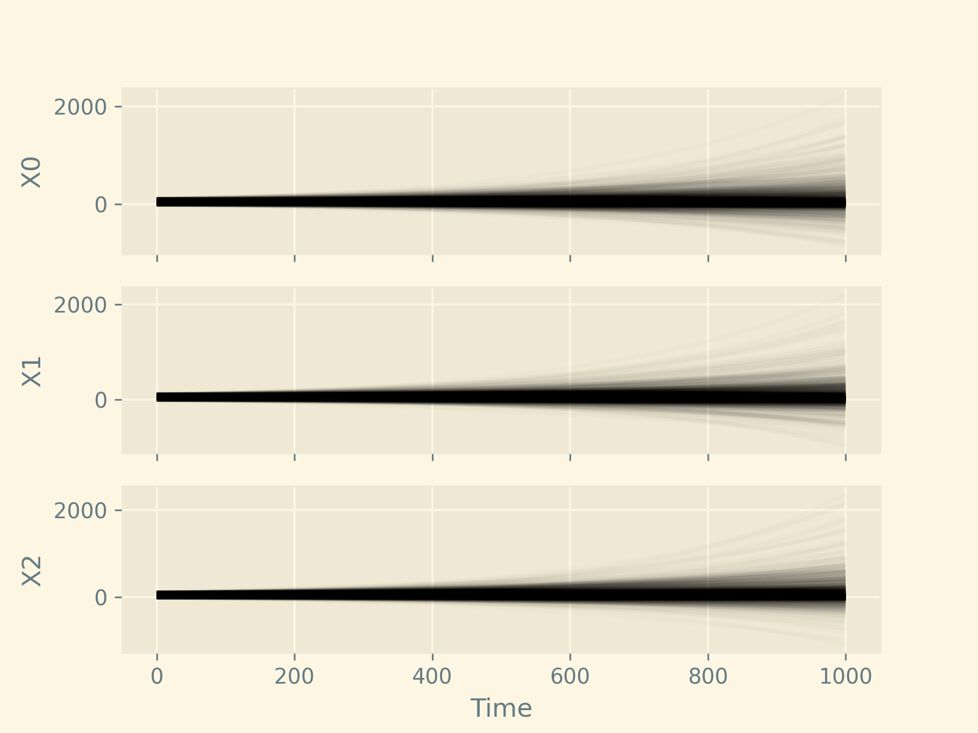
Here is the resulting plot. Since we chose the coefficient distributions somewhat haphazardly, it is should not be surprising that no particular direction was preferred for this system.