A Rust Implementation of the Poisson Binomial Probability Distribution

The probability mass function of the Poisson binomial distribution is given by

\[\sum_{A \in F_k} \prod_{i \in A} p_i \prod_{j \in A^c} (1 - p_j)\]

where \(F_k\) is the set of all subsets of \(k\) integers that can be selected from the set \(\{ 1, \ldots, n \}\). This expression does not by itself suggest one algorithm over another due to the cummutativty and associativity of the operators involved.

Wikipedia gives pseudocode for computing the probability mass function for the Poisson binomial distribution via what it terms the “direct convolution algorithm”.

fn dc(p: &[f64]) -> Vec<f64> {
    let n = p.len();
    let mut pmf: Vec<f64> = vec![1.0]; // PMF array with size 1, initialized to 1

    for i in 0..n {
        // Create a new next_pmf array with size i + 2
        let mut next_pmf: Vec<f64> = vec![0.0; i + 2]; 

        // Calculate the first element of next_pmf
        next_pmf[0] = (1.0 - p[i]) * pmf[0];

        // Calculate the last element of next_pmf if within bounds
        if i < pmf.len() {
            next_pmf[i + 1] = p[i] * pmf[i];
        }

        // Update the rest of next_pmf
        for k in 1..=i {
            next_pmf[k] = p[i] * pmf[k - 1] + (1.0 - p[i]) * pmf[k];
        }

        // Update pmf for the next iteration
        pmf = next_pmf;
    }

    pmf
}

Let’s try to use the algorithm.

// Example usage
let p: Vec<f64> = vec![0.1, 0.2, 0.3, 0.4];
let pmf: Vec<f64> = dc(&p);
println!("{:?}", pmf);

We can also double check that the result resembles a probability by checking if the sum of the probabilities is in fact equal to unity.

let sum_check: f64 = pmf.iter().sum(); // Calculate the sum of the PMF values
println!("Sum of PMF: {}", sum_check);

We can also define the cumulative distribution function (CDF) as the cumulative sum of the PMF.

fn compute_cdf(pmf: &[f64]) -> Vec<f64> {
    let mut cdf: Vec<f64> = Vec::with_capacity(pmf.len());
    let mut sum = 0.0;

    for &prob in pmf {
        sum += prob;
        cdf.push(sum);
    }

    cdf
}

Here is an example of using the CDF.

let cdf: Vec<f64> = compute_cdf(&pmf);
println!("CDF: {:?}", cdf);

Often we will want to be able to sample from such a probability distribution. Here is a function which implicitly relies on the inverse transform theorem.

:dep rand
use rand::Rng;

fn sample_from_distribution(cdf: &[f64]) -> usize {
    let mut rng = rand::thread_rng();
    let random_value: f64 = rng.gen(); // Generate a uniform random value between 0 and 1

    cdf.iter()
        .position(|&x| random_value <= x)
        .unwrap_or(cdf.len() - 1) // If not found, return the last index
}

Now let us take some samples.

let num_samples = 10000;

let samples: Vec<usize> = (0..num_samples)
        .map(|_| sample_from_distribution(&cdf))
        .collect();


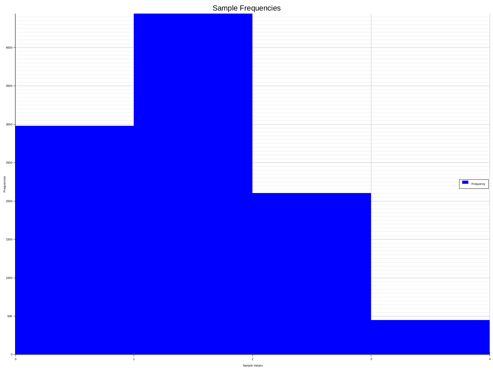
println!("Samples: {:?}", samples);

And finally let’s visualize the sample. In order to do this, let us define a chart using the plotters crate.

:dep plotters
use plotters::prelude::*;

fn plot_histogram(samples: &[usize], filename: &str) {
    let max_value = *samples.iter().max().unwrap_or(&0);
    let frequencies = (0..=max_value)
        .map(|value| samples.iter().filter(|&&x| x == value).count() as u32)
        .collect::<Vec<_>>();

    let root = BitMapBackend::new(filename, (1600, 1200)).into_drawing_area();
    root.fill(&WHITE).unwrap();

    let mut chart = ChartBuilder::on(&root)
        .margin(10)
        .x_label_area_size(40)
        .y_label_area_size(40)
        .caption("Sample Frequencies", ("sans-serif", 30).into_font())
        .build_cartesian_2d(0..max_value, 0..*frequencies.iter().max().unwrap_or(&0))
        .unwrap();

    chart
        .configure_mesh()
        .x_desc("Sample Values")
        .y_desc("Frequencies")
        .draw()
        .unwrap();

    chart
        .draw_series(
            (0..=max_value)
                .map(|x| {
                    let freq = frequencies[x];
                    Rectangle::new(
                        [(x as usize, 0), ((x + 1) as usize, freq)],
                        BLUE.filled(),
                    )
                }),
        )
        .unwrap()
        .label("Frequency")
        .legend(|(x, y)| Rectangle::new([(x, y - 10), (x + 20, y)], BLUE.filled()));

    chart
        .configure_series_labels()
        .border_style(&BLACK)
        .background_style(&WHITE)
        .draw()
        .unwrap();
}

Let’s make the plot.

plot_histogram(&samples, "histogram.png");

Figure 1: Sample frequencies from a Poisson binomial distribution.