When I listen to what people are describing as patterns in the data I rarely find that linearity itself is of any core interest. Rather, many tools and educational resources are oriented around linear models. That itself I think has to do with path-dependence of historical developments and the computational feasibility of fitting linear models. But when pressed I find that most people don’t actually give any special preference to linearity being scientifically plausible.
Now what is going to seem like a weird flex for many people is the notion of being able to do structural equation models (Bollen 1989) on ranks. For other people, who were told from on-high “thou shalt not regress on ranks”, will see this approach as invalid. But it is valid. It’s math.
Structural Model
First, I used a naive algorithm to choose a structural model at random. Here it is in R-like (specifically Lavaan-like) equations (Rosseel 2012):
x42 ~ x90+x0
x27 ~ x87+x32
x12 ~ x0+x3+x84
x74 ~ x83+x76+x50
x63 ~ x51+x44+x77+x28
x93 ~ x90
x30 ~ x97
x14 ~ x44+x54
x81 ~ x6
x38 ~ x23+x49
x29 ~ x9
x62 ~ x2
x75 ~ x57
x31 ~ x65
x71 ~ x15
x68 ~ x87+x65
x43 ~ x1
x92 ~ x1
x60 ~ x96+x37
x0 ~ x5
x3 ~ x44+x89+x37
x50 ~ x16
x90 ~ x80
x2 ~ x67+x10
x57 ~ x65+x67+x7+x26
x1 ~ x66+x40
x96 ~ x4+x55
x5 ~ x41
x44 ~ x55
x89 ~ x15+x55
x37 ~ x54
x10 ~ x25+x52+x16
x67 ~ x84
x66 ~ x47+x22
x4 ~ x77
x54 ~ x87+x85
x25 ~ x19
x52 ~ x83
x47 ~ x13+x70
x22 ~ x7+x28
x87 ~ x16+x88+x78+x64
x19 ~ x58
x83 ~ x61
x13 ~ x58
x70 ~ x97+x80
x7 ~ x23
x88 ~ x6
x64 ~ x9
x61 ~ x84
x58 ~ x17
x23 ~ x59+x94
x9 ~ x78+x36
x17 ~ x79
x59 ~ x55
x79 ~ x77+x26
x55 ~ x20+x6+x33
x77 ~ x41
x26 ~ x84
x20 ~ x72
x84 ~ x98+x72
x72 ~ x82
x82 ~ x8
Pretty incomprehensible, right? Well, that’s not the syntax’s fault. And it isn’t entirely the fault of my not sorting the order of the equations, although that could have helped. This is a pretty complicated model! We’ll look at the results momentarily. Next I used a choice of sampling distribution to generate the data according to the structural equation model under an assumption of normality.
Each variable \(X_j\) in structural form was simply of the form
\[X_j = \sum_{i \in \text{parents}(j)} \beta_{ij} X_i + \epsilon_j\]
where \(\text{parents}(j)\) represents the set of parent nodes in the directed graph and I took
\[\epsilon_j \sim \mathcal{N}(0,1)\]
and
\[\beta_{ij} \sim \mathcal{N}(0,10).\]
Note that when \(j\) does not have any parents in the graph that implies that
\[X_j = \epsilon_j\]
meaning that (1) our variables are already standardized and (2) this is a pretty run-of-the-mill linear SEM that induces (via change of variables) a multivariate normal distribution over the random variables \[\{ X_0, \ldots, X_{99} \}\].
Train Linear SEM
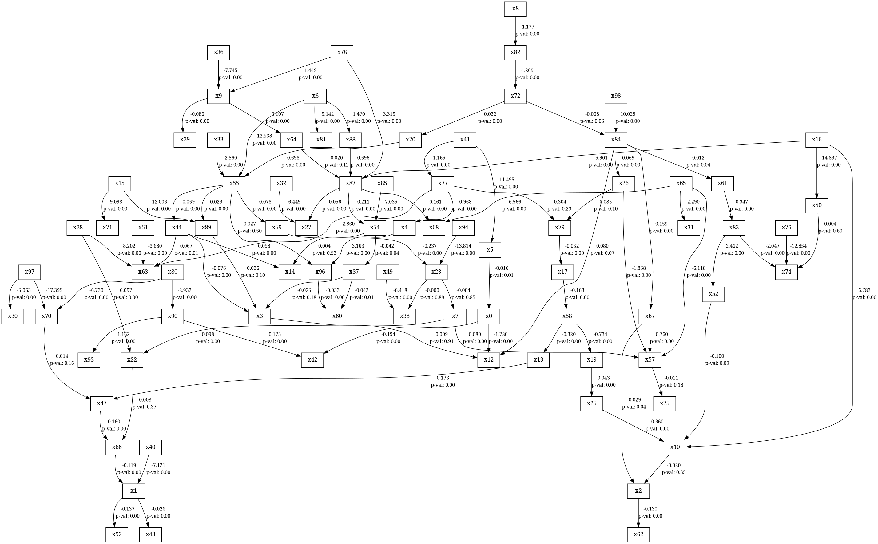
Ignore the p-values in this example. We don’t care about those in this post, and they’re not the right p-values anyway.
| lval | op | rval | Estimate | Std. Err | z-value | p-value |
|---|---|---|---|---|---|---|
| x0 | ~ | x5 | -0.0158832 | 0.00651196 | -2.43908 | 0.0147246 |
| x3 | ~ | x44 | -0.0756279 | 0.0259957 | -2.90925 | 0.00362303 |
| x3 | ~ | x89 | 0.0258967 | 0.0155262 | 1.66793 | 0.0953292 |
| x3 | ~ | x37 | -0.0249739 | 0.0184324 | -1.35489 | 0.175452 |
| x50 | ~ | x16 | -14.8368 | 0.0322415 | -460.179 | 0 |
| x90 | ~ | x80 | -2.93151 | 0.0320633 | -91.4287 | 0 |
| x2 | ~ | x67 | -0.0292056 | 0.0143646 | -2.03316 | 0.042036 |
| x2 | ~ | x10 | -0.0202138 | 0.0216339 | -0.934354 | 0.350122 |
| x57 | ~ | x65 | -6.11732 | 0.428089 | -14.2898 | 0 |
| x57 | ~ | x67 | 0.760306 | 0.0233431 | 32.5709 | 0 |
| x57 | ~ | x7 | 0.0803973 | 0.0241183 | 3.33346 | 0.000857734 |
| x57 | ~ | x26 | -1.858 | 0.056646 | -32.8003 | 0 |
| x1 | ~ | x66 | -0.118996 | 0.0200425 | -5.93719 | 2.89951e-09 |
| x1 | ~ | x40 | -7.12147 | 0.121875 | -58.4324 | 0 |
| x96 | ~ | x4 | 3.16283 | 0.229647 | 13.7726 | 0 |
| x96 | ~ | x55 | 0.0274288 | 0.0408267 | 0.671835 | 0.501689 |
| x5 | ~ | x41 | -11.4945 | 0.0321778 | -357.219 | 0 |
| x44 | ~ | x55 | -0.0593373 | 0.0164798 | -3.60061 | 0.000317471 |
| x89 | ~ | x15 | -12.0029 | 0.104779 | -114.554 | 0 |
| x89 | ~ | x55 | 0.0234407 | 0.00738285 | 3.17503 | 0.00149823 |
| x37 | ~ | x54 | -0.0420312 | 0.0203518 | -2.06523 | 0.0389008 |
| x10 | ~ | x25 | 0.359585 | 0.0598 | 6.01313 | 1.81979e-09 |
| x10 | ~ | x52 | -0.0998501 | 0.0590903 | -1.68979 | 0.0910684 |
| x10 | ~ | x16 | 6.78323 | 0.325214 | 20.8577 | 0 |
| x67 | ~ | x84 | 0.159328 | 0.0563247 | 2.82873 | 0.00467326 |
| x66 | ~ | x47 | 0.159663 | 0.031331 | 5.09601 | 3.46878e-07 |
| x66 | ~ | x22 | -0.00835746 | 0.00933564 | -0.895221 | 0.370669 |
| x4 | ~ | x77 | -0.967856 | 0.0405739 | -23.8541 | 0 |
| x54 | ~ | x87 | 0.211509 | 0.0636722 | 3.32184 | 0.000894271 |
| x54 | ~ | x85 | 7.0352 | 0.463738 | 15.1706 | 0 |
| x25 | ~ | x19 | 0.043103 | 0.014441 | 2.98476 | 0.00283799 |
| x52 | ~ | x83 | 2.46168 | 0.0793286 | 31.0314 | 0 |
| x47 | ~ | x13 | 0.176316 | 0.0362993 | 4.85729 | 1.19002e-06 |
| x47 | ~ | x70 | 0.0139711 | 0.00987645 | 1.41459 | 0.157188 |
| x22 | ~ | x7 | 0.0976122 | 0.0346553 | 2.81666 | 0.0048526 |
| x22 | ~ | x28 | 6.09568 | 0.620052 | 9.83092 | 0 |
| x87 | ~ | x16 | -5.90051 | 0.0788379 | -74.8436 | 0 |
| x87 | ~ | x88 | -0.595774 | 0.042375 | -14.0596 | 0 |
| x87 | ~ | x78 | 3.31886 | 0.0739847 | 44.8588 | 0 |
| x87 | ~ | x64 | 0.0195912 | 0.0125143 | 1.56551 | 0.117464 |
| x19 | ~ | x58 | -0.733988 | 0.0804946 | -9.11848 | 0 |
| x83 | ~ | x61 | 0.347471 | 0.0243161 | 14.2897 | 0 |
| x13 | ~ | x58 | -0.320342 | 0.0365891 | -8.75514 | 0 |
| x70 | ~ | x97 | -17.3946 | 0.0294302 | -591.046 | 0 |
| x70 | ~ | x80 | -6.73016 | 0.0318525 | -211.291 | 0 |
| x7 | ~ | x23 | -0.00418637 | 0.0214885 | -0.194819 | 0.845535 |
| x88 | ~ | x6 | 1.46973 | 0.0301277 | 48.7835 | 0 |
| x64 | ~ | x9 | 0.107246 | 0.0243442 | 4.40542 | 1.0558e-05 |
| x61 | ~ | x84 | 0.0115246 | 0.00556868 | 2.06954 | 0.0384957 |
| x58 | ~ | x17 | -0.163472 | 0.0237576 | -6.88082 | 5.9508e-12 |
| x23 | ~ | x59 | -0.236768 | 0.0679229 | -3.48583 | 0.000490618 |
| x23 | ~ | x94 | -13.8165 | 0.703749 | -19.6327 | 0 |
| x9 | ~ | x78 | 1.44856 | 0.0309672 | 46.7773 | 0 |
| x9 | ~ | x36 | -7.74544 | 0.0324563 | -238.642 | 0 |
| x17 | ~ | x79 | -0.0515049 | 0.014378 | -3.58219 | 0.00034072 |
| x59 | ~ | x55 | -0.0778839 | 0.0232169 | -3.35463 | 0.000794725 |
| x79 | ~ | x77 | -0.304188 | 0.254101 | -1.19711 | 0.231262 |
| x79 | ~ | x26 | 0.0846485 | 0.0518044 | 1.634 | 0.102258 |
| x55 | ~ | x20 | 0.698485 | 0.0441722 | 15.8128 | 0 |
| x55 | ~ | x6 | 12.5385 | 0.106001 | 118.286 | 0 |
| x55 | ~ | x33 | 2.56006 | 0.110402 | 23.1886 | 0 |
| x77 | ~ | x41 | -1.16488 | 0.0334789 | -34.7944 | 0 |
| x26 | ~ | x84 | 0.0692953 | 0.0232002 | 2.98685 | 0.00281871 |
| x20 | ~ | x72 | 0.0218056 | 0.00738758 | 2.95166 | 0.00316072 |
| x84 | ~ | x98 | 10.0285 | 0.04488 | 223.452 | 0 |
| x84 | ~ | x72 | -0.00825119 | 0.00430194 | -1.91802 | 0.0551089 |
| x72 | ~ | x82 | 4.26913 | 0.171663 | 24.8693 | 0 |
| x82 | ~ | x8 | -1.177 | 0.0307035 | -38.3345 | 0 |
| x42 | ~ | x90 | 0.174795 | 0.0225525 | 7.75057 | 9.10383e-15 |
| x42 | ~ | x0 | -0.193506 | 0.0288042 | -6.71797 | 1.84273e-11 |
| x27 | ~ | x87 | -0.0558945 | 0.0155562 | -3.59307 | 0.000326803 |
| x27 | ~ | x32 | -6.44944 | 0.11109 | -58.0559 | 0 |
| x12 | ~ | x0 | -1.77993 | 0.19173 | -9.28355 | 0 |
| x12 | ~ | x3 | 0.00869965 | 0.0739928 | 0.117574 | 0.906405 |
| x12 | ~ | x84 | 0.0798634 | 0.0436139 | 1.83115 | 0.0670785 |
| x74 | ~ | x83 | -2.04682 | 0.0658169 | -31.0987 | 0 |
| x74 | ~ | x76 | -12.8538 | 0.0962878 | -133.494 | 0 |
| x74 | ~ | x50 | 0.00363404 | 0.00693041 | 0.524361 | 0.600028 |
| x63 | ~ | x51 | -3.6804 | 0.180348 | -20.4072 | 0 |
| x63 | ~ | x44 | 0.0674865 | 0.0257225 | 2.62364 | 0.00869956 |
| x63 | ~ | x77 | -2.86011 | 0.121978 | -23.4479 | 0 |
| x63 | ~ | x28 | 8.20213 | 0.189614 | 43.2569 | 0 |
| x93 | ~ | x90 | 1.16241 | 0.126722 | 9.1729 | 0 |
| x30 | ~ | x97 | -5.06266 | 0.0305478 | -165.729 | 0 |
| x14 | ~ | x44 | 0.0582553 | 0.0131839 | 4.41866 | 9.93166e-06 |
| x14 | ~ | x54 | 0.00383844 | 0.00602918 | 0.636644 | 0.524357 |
| x81 | ~ | x6 | 9.14242 | 0.029405 | 310.914 | 0 |
| x38 | ~ | x23 | -0.000191771 | 0.00135337 | -0.141698 | 0.887318 |
| x38 | ~ | x49 | -6.41838 | 0.0346079 | -185.46 | 0 |
| x29 | ~ | x9 | -0.0859488 | 0.0194305 | -4.42339 | 9.71627e-06 |
| x62 | ~ | x2 | -0.130319 | 0.0391703 | -3.32698 | 0.000877925 |
| x75 | ~ | x57 | -0.0106346 | 0.007978 | -1.33299 | 0.182536 |
| x31 | ~ | x65 | 2.29004 | 0.0308554 | 74.2186 | 0 |
| x71 | ~ | x15 | -9.09815 | 0.0328499 | -276.961 | 0 |
| x68 | ~ | x87 | -0.160788 | 0.046685 | -3.44412 | 0.00057293 |
| x68 | ~ | x65 | -6.56613 | 0.332406 | -19.7533 | 0 |
| x43 | ~ | x1 | -0.0262926 | 0.00846914 | -3.10452 | 0.0019059 |
| x92 | ~ | x1 | -0.136973 | 0.0333884 | -4.10242 | 4.08843e-05 |
| x60 | ~ | x96 | -0.0327555 | 0.0081783 | -4.00517 | 6.19727e-05 |
| x60 | ~ | x37 | -0.0417641 | 0.0155725 | -2.68192 | 0.00732005 |
| x1 | x1 | 15.0869 | 0.674707 | 22.3607 | 0 | |
| x72 | x72 | 69.2405 | 3.09653 | 22.3607 | 0 | |
| x88 | x88 | 0.976494 | 0.0436701 | 22.3607 | 0 | |
| x79 | x79 | 153.927 | 6.88384 | 22.3607 | 0 | |
| x37 | x37 | 106.153 | 4.74733 | 22.3607 | 0 | |
| x4 | x4 | 3.92461 | 0.175514 | 22.3607 | 0 | |
| x83 | x83 | 1.94489 | 0.0869781 | 22.3607 | 0 | |
| x26 | x26 | 56.8494 | 2.54238 | 22.3607 | 0 | |
| x20 | x20 | 6.11607 | 0.273519 | 22.3607 | 0 | |
| x10 | x10 | 101.017 | 4.51761 | 22.3607 | 0 | |
| x57 | x57 | 184.031 | 8.2301 | 22.3607 | 0 | |
| x54 | x54 | 206.392 | 9.23014 | 22.3607 | 0 | |
| x84 | x84 | 2.07379 | 0.0927426 | 22.3607 | 0 | |
| x55 | x55 | 12.0374 | 0.53833 | 22.3607 | 0 | |
| x77 | x77 | 1.0784 | 0.0482277 | 22.3607 | 0 | |
| x87 | x87 | 5.9201 | 0.264755 | 22.3607 | 0 | |
| x0 | x0 | 5.43293 | 0.242968 | 22.3607 | 0 | |
| x17 | x17 | 31.9515 | 1.42891 | 22.3607 | 0 | |
| x64 | x64 | 37.1091 | 1.65957 | 22.3607 | 0 | |
| x47 | x47 | 36.3327 | 1.62485 | 22.3607 | 0 | |
| x13 | x13 | 25.6109 | 1.14536 | 22.3607 | 0 | |
| x58 | x58 | 18.2656 | 0.816861 | 22.3607 | 0 | |
| x70 | x70 | 0.940051 | 0.0420404 | 22.3607 | 0 | |
| x67 | x67 | 335.075 | 14.985 | 22.3607 | 0 | |
| x52 | x52 | 14.7385 | 0.659124 | 22.3607 | 0 | |
| x66 | x66 | 36.5782 | 1.63583 | 22.3607 | 0 | |
| x9 | x9 | 1.03993 | 0.0465069 | 22.3607 | 0 | |
| x7 | x7 | 316.36 | 14.148 | 22.3607 | 0 | |
| x22 | x22 | 379.959 | 16.9923 | 22.3607 | 0 | |
| x59 | x59 | 105.018 | 4.69656 | 22.3607 | 0 | |
| x5 | x5 | 0.996211 | 0.0445519 | 22.3607 | 0 | |
| x50 | x50 | 0.992855 | 0.0444018 | 22.3607 | 0 | |
| x25 | x25 | 27.9987 | 1.25214 | 22.3607 | 0 | |
| x44 | x44 | 52.9128 | 2.36633 | 22.3607 | 0 | |
| x3 | x3 | 36.2197 | 1.6198 | 22.3607 | 0 | |
| x89 | x89 | 10.614 | 0.474673 | 22.3607 | 0 | |
| x61 | x61 | 3.27529 | 0.146475 | 22.3607 | 0 | |
| x23 | x23 | 489.941 | 21.9108 | 22.3607 | 0 | |
| x90 | x90 | 0.952558 | 0.0425997 | 22.3607 | 0 | |
| x2 | x2 | 69.6932 | 3.11677 | 22.3607 | 0 | |
| x82 | x82 | 0.951468 | 0.0425509 | 22.3607 | 0 | |
| x96 | x96 | 324.701 | 14.5211 | 22.3607 | 0 | |
| x19 | x19 | 123.953 | 5.54333 | 22.3607 | 0 | |
| x12 | x12 | 200.904 | 8.98471 | 22.3607 | 0 | |
| x74 | x74 | 10.1453 | 0.453714 | 22.3607 | 0 | |
| x27 | x27 | 12.306 | 0.55034 | 22.3607 | 0 | |
| x31 | x31 | 0.956058 | 0.0427562 | 22.3607 | 0 | |
| x62 | x62 | 107.466 | 4.80601 | 22.3607 | 0 | |
| x81 | x81 | 0.930211 | 0.0416003 | 22.3607 | 0 | |
| x29 | x29 | 23.6406 | 1.05724 | 22.3607 | 0 | |
| x60 | x60 | 25.8522 | 1.15614 | 22.3607 | 0 | |
| x92 | x92 | 74.8386 | 3.34688 | 22.3607 | 0 | |
| x14 | x14 | 9.31632 | 0.416639 | 22.3607 | 0 | |
| x42 | x42 | 4.53438 | 0.202784 | 22.3607 | 0 | |
| x38 | x38 | 1.25457 | 0.0561059 | 22.3607 | 0 | |
| x75 | x75 | 39.0543 | 1.74656 | 22.3607 | 0 | |
| x93 | x93 | 143.164 | 6.40249 | 22.3607 | 0 | |
| x68 | x68 | 110.951 | 4.96189 | 22.3607 | 0 | |
| x71 | x71 | 1.04381 | 0.0466808 | 22.3607 | 0 | |
| x43 | x43 | 4.8152 | 0.215342 | 22.3607 | 0 | |
| x63 | x63 | 35.463 | 1.58595 | 22.3607 | 0 | |
| x30 | x30 | 1.01283 | 0.0452951 | 22.3607 | 0 |
Train Rank SEM
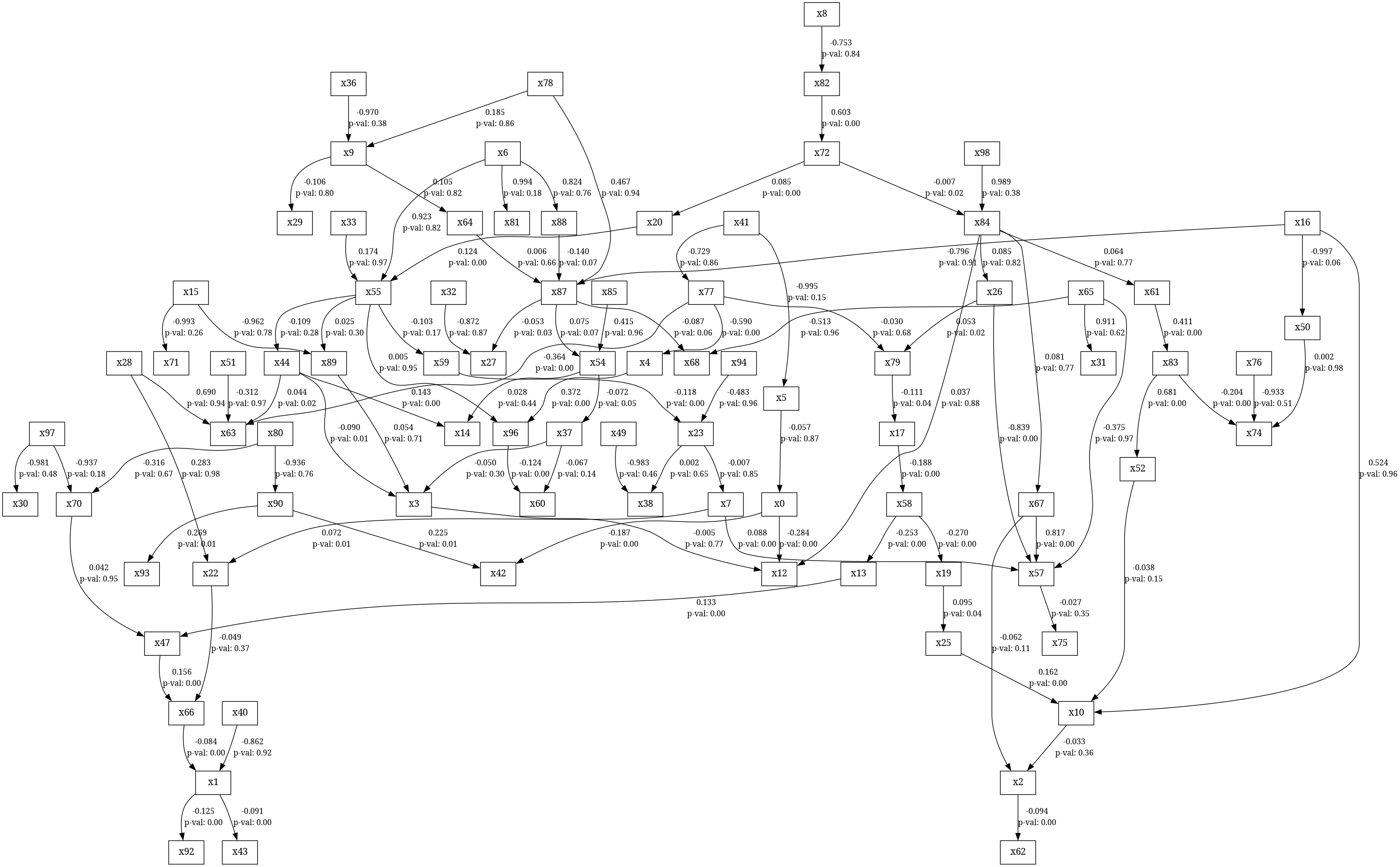
Now let’s look at the result on the ranks.
| lval | op | rval | Estimate | Std. Err | z-value | p-value |
|---|---|---|---|---|---|---|
| x0 | ~ | x5 | -0.0506852 | 0.319554 | -0.158612 | 0.873974 |
| x3 | ~ | x44 | -0.090607 | 0.035594 | -2.54557 | 0.01091 |
| x3 | ~ | x89 | 0.0528289 | 0.178962 | 0.295197 | 0.767844 |
| x3 | ~ | x37 | -0.0489985 | 0.0467657 | -1.04774 | 0.294757 |
| x50 | ~ | x16 | -0.997288 | 0.642918 | -1.55119 | 0.120856 |
| x90 | ~ | x80 | -0.935912 | 2.32397 | -0.40272 | 0.687154 |
| x2 | ~ | x67 | -0.0623613 | 0.0343197 | -1.81707 | 0.0692058 |
| x2 | ~ | x10 | -0.0366353 | 0.0363691 | -1.00732 | 0.313781 |
| x57 | ~ | x65 | -0.376144 | 9.81514 | -0.0383228 | 0.96943 |
| x57 | ~ | x67 | 0.808757 | 0.028215 | 28.6641 | 0 |
| x57 | ~ | x7 | 0.0879096 | 0.0286485 | 3.06856 | 0.00215096 |
| x57 | ~ | x26 | -0.832015 | 0.0240271 | -34.6282 | 0 |
| x1 | ~ | x66 | -0.084396 | 0.0165049 | -5.11339 | 3.16423e-07 |
| x1 | ~ | x40 | -0.860226 | 7.79065 | -0.110418 | 0.912078 |
| x96 | ~ | x4 | 0.371961 | 0.0457266 | 8.13446 | 4.44089e-16 |
| x96 | ~ | x55 | 0.00506802 | 0.0736767 | 0.0687872 | 0.945159 |
| x5 | ~ | x41 | -0.995247 | 0.838395 | -1.18709 | 0.235194 |
| x44 | ~ | x55 | -0.110851 | 0.0950145 | -1.16668 | 0.24334 |
| x89 | ~ | x15 | -0.961625 | 2.68861 | -0.357666 | 0.720593 |
| x89 | ~ | x55 | 0.0254901 | 0.0188921 | 1.34925 | 0.177257 |
| x37 | ~ | x54 | -0.0709773 | 0.0357109 | -1.98755 | 0.0468613 |
| x10 | ~ | x25 | 0.164821 | 0.021529 | 7.65575 | 1.93179e-14 |
| x10 | ~ | x52 | -0.0448535 | 0.0272714 | -1.64471 | 0.10003 |
| x10 | ~ | x16 | 0.524877 | 10.3321 | 0.0508006 | 0.959484 |
| x67 | ~ | x84 | 0.0815371 | 0.273401 | 0.298233 | 0.765525 |
| x66 | ~ | x47 | 0.157112 | 0.0312812 | 5.02256 | 5.09866e-07 |
| x66 | ~ | x22 | -0.0479852 | 0.0520462 | -0.921973 | 0.356543 |
| x4 | ~ | x77 | -0.590027 | 0.0522867 | -11.2845 | 0 |
| x54 | ~ | x87 | 0.0743098 | 0.044113 | 1.68453 | 0.0920785 |
| x54 | ~ | x85 | 0.415275 | 9.12442 | 0.0455125 | 0.963699 |
| x25 | ~ | x19 | 0.0915282 | 0.0455169 | 2.01086 | 0.0443403 |
| x52 | ~ | x83 | 0.681846 | 0.0406469 | 16.7749 | 0 |
| x47 | ~ | x13 | 0.133902 | 0.0320736 | 4.17484 | 2.98197e-05 |
| x47 | ~ | x70 | 0.041785 | 0.504127 | 0.0828859 | 0.933942 |
| x22 | ~ | x7 | 0.07196 | 0.0261834 | 2.74831 | 0.00599034 |
| x22 | ~ | x28 | 0.282929 | 9.04255 | 0.0312886 | 0.975039 |
| x87 | ~ | x16 | -0.796425 | 6.55258 | -0.121544 | 0.90326 |
| x87 | ~ | x88 | -0.139354 | 0.0835817 | -1.66728 | 0.0954584 |
| x87 | ~ | x78 | 0.465273 | 6.14948 | 0.0756605 | 0.939689 |
| x87 | ~ | x64 | 0.00794462 | 0.0136198 | 0.583315 | 0.559681 |
| x19 | ~ | x58 | -0.269086 | 0.0193834 | -13.8823 | 0 |
| x83 | ~ | x61 | 0.40993 | 0.0318307 | 12.8784 | 0 |
| x13 | ~ | x58 | -0.250342 | 0.0291525 | -8.5873 | 0 |
| x70 | ~ | x97 | -0.937119 | 0.895642 | -1.04631 | 0.295418 |
| x70 | ~ | x80 | -0.315995 | 0.969359 | -0.325984 | 0.744437 |
| x7 | ~ | x23 | -0.00693939 | 0.0356268 | -0.19478 | 0.845565 |
| x88 | ~ | x6 | 0.823842 | 2.33363 | 0.35303 | 0.724066 |
| x64 | ~ | x9 | 0.10536 | 0.360136 | 0.292557 | 0.769861 |
| x61 | ~ | x84 | 0.0647399 | 0.183626 | 0.352563 | 0.724416 |
| x58 | ~ | x17 | -0.190366 | 0.0315347 | -6.03673 | 1.57271e-09 |
| x23 | ~ | x59 | -0.118138 | 0.0298934 | -3.95198 | 7.75065e-05 |
| x23 | ~ | x94 | -0.482748 | 9.61376 | -0.0502143 | 0.959952 |
| x9 | ~ | x78 | 0.184565 | 1.25217 | 0.147397 | 0.882819 |
| x9 | ~ | x36 | -0.969891 | 1.31238 | -0.739033 | 0.459887 |
| x17 | ~ | x79 | -0.108698 | 0.0513214 | -2.11798 | 0.0341769 |
| x59 | ~ | x55 | -0.100981 | 0.0721987 | -1.39866 | 0.161916 |
| x79 | ~ | x77 | -0.0331926 | 0.072199 | -0.459737 | 0.645705 |
| x79 | ~ | x26 | 0.054813 | 0.0226565 | 2.4193 | 0.0155503 |
| x55 | ~ | x20 | 0.122512 | 0.0186636 | 6.56418 | 5.23206e-11 |
| x55 | ~ | x6 | 0.923404 | 4.18694 | 0.220544 | 0.825448 |
| x55 | ~ | x33 | 0.174377 | 4.36078 | 0.0399877 | 0.968103 |
| x77 | ~ | x41 | -0.72968 | 4.14135 | -0.176194 | 0.860142 |
| x26 | ~ | x84 | 0.084089 | 0.321057 | 0.261913 | 0.793389 |
| x20 | ~ | x72 | 0.0890476 | 0.0201729 | 4.41421 | 1.01379e-05 |
| x84 | ~ | x98 | 0.989211 | 1.25365 | 0.789063 | 0.430075 |
| x84 | ~ | x72 | -0.0069965 | 0.00352878 | -1.9827 | 0.0474011 |
| x72 | ~ | x82 | 0.599442 | 0.094153 | 6.36668 | 1.93166e-10 |
| x82 | ~ | x8 | -0.752035 | 3.73609 | -0.201289 | 0.840472 |
| x42 | ~ | x90 | 0.223544 | 0.0999267 | 2.23708 | 0.0252814 |
| x42 | ~ | x0 | -0.187517 | 0.026882 | -6.97555 | 3.04667e-12 |
| x27 | ~ | x87 | -0.054163 | 0.0249817 | -2.1681 | 0.0301507 |
| x27 | ~ | x32 | -0.871473 | 5.06653 | -0.172006 | 0.863433 |
| x12 | ~ | x0 | -0.283938 | 0.0358551 | -7.91903 | 2.44249e-15 |
| x12 | ~ | x3 | -0.0053715 | 0.0198303 | -0.270873 | 0.786488 |
| x12 | ~ | x84 | 0.0369434 | 0.233865 | 0.157969 | 0.874481 |
| x74 | ~ | x83 | -0.203575 | 0.00701163 | -29.034 | 0 |
| x74 | ~ | x76 | -0.932689 | 1.70561 | -0.546837 | 0.584491 |
| x74 | ~ | x50 | 0.00199484 | 0.0896919 | 0.022241 | 0.982256 |
| x63 | ~ | x51 | -0.308836 | 7.64331 | -0.0404061 | 0.967769 |
| x63 | ~ | x44 | 0.042995 | 0.0189662 | 2.26693 | 0.0233946 |
| x63 | ~ | x77 | -0.364178 | 0.062133 | -5.86126 | 4.59371e-09 |
| x63 | ~ | x28 | 0.689741 | 8.03641 | 0.085827 | 0.931604 |
| x93 | ~ | x90 | 0.269947 | 0.130042 | 2.07584 | 0.0379089 |
| x30 | ~ | x97 | -0.980854 | 1.60828 | -0.609879 | 0.541942 |
| x14 | ~ | x44 | 0.141669 | 0.0227724 | 6.22108 | 4.9375e-10 |
| x14 | ~ | x54 | 0.0268343 | 0.0338546 | 0.792634 | 0.427991 |
| x81 | ~ | x6 | 0.99423 | 0.896012 | 1.10962 | 0.267165 |
| x38 | ~ | x23 | 0.00220938 | 0.00520095 | 0.424803 | 0.67098 |
| x38 | ~ | x49 | -0.982967 | 1.54838 | -0.634837 | 0.525535 |
| x29 | ~ | x9 | -0.0979993 | 0.331924 | -0.295246 | 0.767806 |
| x62 | ~ | x2 | -0.0934138 | 0.0264644 | -3.52979 | 0.000415892 |
| x75 | ~ | x57 | -0.0275633 | 0.0272089 | -1.01302 | 0.311049 |
| x31 | ~ | x65 | 0.911065 | 1.97102 | 0.46223 | 0.643916 |
| x71 | ~ | x15 | -0.992771 | 0.986135 | -1.00673 | 0.314065 |
| x68 | ~ | x87 | -0.0876041 | 0.0452074 | -1.93783 | 0.0526445 |
| x68 | ~ | x65 | -0.512031 | 9.14152 | -0.0560116 | 0.955333 |
| x43 | ~ | x1 | -0.0896154 | 0.0247739 | -3.61733 | 0.000297661 |
| x92 | ~ | x1 | -0.127711 | 0.045804 | -2.7882 | 0.00530012 |
| x60 | ~ | x96 | -0.122361 | 0.0423403 | -2.88994 | 0.00385318 |
| x60 | ~ | x37 | -0.0640426 | 0.0445107 | -1.43881 | 0.150203 |
| x1 | x1 | 61647.5 | 2756.96 | 22.3607 | 0 | |
| x72 | x72 | 124894 | 5585.41 | 22.3607 | 0 | |
| x88 | x88 | 5858.72 | 262.01 | 22.3607 | 0 | |
| x79 | x79 | 86020 | 3846.93 | 22.3607 | 0 | |
| x37 | x37 | 102190 | 4570.06 | 22.3607 | 0 | |
| x4 | x4 | 45114.9 | 2017.6 | 22.3607 | 0 | |
| x83 | x83 | 55543.9 | 2484 | 22.3607 | 0 | |
| x26 | x26 | 167565 | 7493.74 | 22.3607 | 0 | |
| x20 | x20 | 52885.3 | 2365.1 | 22.3607 | 0 | |
| x10 | x10 | 101961 | 4559.83 | 22.3607 | 0 | |
| x57 | x57 | 96742.2 | 4326.44 | 22.3607 | 0 | |
| x54 | x54 | 79904.8 | 3573.45 | 22.3607 | 0 | |
| x84 | x84 | 1618.25 | 72.3703 | 22.3607 | 0 | |
| x55 | x55 | 18780.6 | 839.893 | 22.3607 | 0 | |
| x77 | x77 | 16501.5 | 737.97 | 22.3607 | 0 | |
| x87 | x87 | 40933.5 | 1830.6 | 22.3607 | 0 | |
| x0 | x0 | 69157.1 | 3092.8 | 22.3607 | 0 | |
| x17 | x17 | 227941 | 10193.8 | 22.3607 | 0 | |
| x64 | x64 | 220649 | 9867.73 | 22.3607 | 0 | |
| x47 | x47 | 221531 | 9907.18 | 22.3607 | 0 | |
| x13 | x13 | 200558 | 8969.24 | 22.3607 | 0 | |
| x58 | x58 | 227689 | 10182.6 | 22.3607 | 0 | |
| x70 | x70 | 870.628 | 38.9357 | 22.3607 | 0 | |
| x67 | x67 | 121512 | 5434.17 | 22.3607 | 0 | |
| x52 | x52 | 106988 | 4784.65 | 22.3607 | 0 | |
| x66 | x66 | 220552 | 9863.37 | 22.3607 | 0 | |
| x9 | x9 | 1700.29 | 76.0391 | 22.3607 | 0 | |
| x7 | x7 | 117868 | 5271.21 | 22.3607 | 0 | |
| x22 | x22 | 80809.7 | 3613.92 | 22.3607 | 0 | |
| x59 | x59 | 102120 | 4566.94 | 22.3607 | 0 | |
| x5 | x5 | 676.295 | 30.2448 | 22.3607 | 0 | |
| x50 | x50 | 394.791 | 17.6556 | 22.3607 | 0 | |
| x25 | x25 | 219095 | 9798.21 | 22.3607 | 0 | |
| x44 | x44 | 176861 | 7909.45 | 22.3607 | 0 | |
| x3 | x3 | 224375 | 10034.4 | 22.3607 | 0 | |
| x89 | x89 | 6992.15 | 312.698 | 22.3607 | 0 | |
| x61 | x61 | 54813.7 | 2451.34 | 22.3607 | 0 | |
| x23 | x23 | 91434.3 | 4089.07 | 22.3607 | 0 | |
| x90 | x90 | 5004.22 | 223.796 | 22.3607 | 0 | |
| x2 | x2 | 143134 | 6401.15 | 22.3607 | 0 | |
| x82 | x82 | 14088.2 | 630.042 | 22.3607 | 0 | |
| x96 | x96 | 106344 | 4755.84 | 22.3607 | 0 | |
| x19 | x19 | 88664.1 | 3965.18 | 22.3607 | 0 | |
| x12 | x12 | 88909.9 | 3976.17 | 22.3607 | 0 | |
| x74 | x74 | 3183.6 | 142.375 | 22.3607 | 0 | |
| x27 | x27 | 25626.2 | 1146.04 | 22.3607 | 0 | |
| x31 | x31 | 3901.27 | 174.47 | 22.3607 | 0 | |
| x62 | x62 | 100679 | 4502.49 | 22.3607 | 0 | |
| x81 | x81 | 863.707 | 38.6262 | 22.3607 | 0 | |
| x29 | x29 | 187434 | 8382.29 | 22.3607 | 0 | |
| x60 | x60 | 203258 | 9089.98 | 22.3607 | 0 | |
| x92 | x92 | 132720 | 5935.43 | 22.3607 | 0 | |
| x14 | x14 | 91841.5 | 4107.28 | 22.3607 | 0 | |
| x42 | x42 | 49977 | 2235.04 | 22.3607 | 0 | |
| x38 | x38 | 2511.92 | 112.337 | 22.3607 | 0 | |
| x75 | x75 | 217012 | 9705.05 | 22.3607 | 0 | |
| x93 | x93 | 84640.2 | 3785.22 | 22.3607 | 0 | |
| x68 | x68 | 83919 | 3752.97 | 22.3607 | 0 | |
| x71 | x71 | 940.648 | 42.0671 | 22.3607 | 0 | |
| x43 | x43 | 38825.7 | 1736.34 | 22.3607 | 0 | |
| x63 | x63 | 63706.2 | 2849.03 | 22.3607 | 0 | |
| x30 | x30 | 2807.35 | 125.548 | 22.3607 | 0 |
Python Code
If you want to tinker around with the above example, here is the Python code.
from itertools import product
import random

import matplotlib.pyplot as plt
import networkx as nx
import numpy as np
import pandas as pd
from scipy.stats import rankdata
import semopy

# Utils

def decycle(d):
    '''
    Pseudorandomly remove cycles from a directed graph.

    Changes the graph inplace.

    PARAMETERS
    ----------
    d : networkx.DiGraph
        Directed graph.

    RETURNS
    -------
    None
    '''
    while True:
        if nx.is_directed_acyclic_graph(d):
            break
        first_cycle = nx.cycles.find_cycle(d)
        target_edge = random.sample(first_cycle, 1)[0]
        d.remove_edge(*target_edge)

rank = lambda x: rankdata(x, method='dense', axis=0)

# Config
n = 100
m = 1000
possible_edges = list(product(range(n), repeat=2))
np.random.seed(2018)

# Generate a DAG
d = nx.DiGraph()
edges = random.sample(possible_edges, n)
d.add_edges_from(edges)
decycle(d)

# Create Lavaan-style string following DAG
model_str = ''
for node in nx.topological_sort(d):
    node_str = f''
    for i, edge in enumerate(d.out_edges(node)):
        if i == 0:
            node_str += f'x{edge[1]}'
        else:
            node_str += f'+x{edge[1]}'
    if node_str:
        model_str += f'x{node} ~ {node_str}\n'

print(model_str)
model = semopy.Model(model_str)


# Generate data that follows DAG
data = np.random.normal(size=m*n).reshape(m,n)
betas = {edge:np.random.normal(scale=10) for edge in d.edges()}
for node in nx.topological_sort(d):
    for edge in d.out_edges(node):
        data[:,node] += betas[edge] * data[:,edge[1]]

df = pd.DataFrame(data, columns=[f'x{i}' for i in range(n)])
df_rank = pd.DataFrame(rank(data), columns=[f'x{i}' for i in range(n)])

# Train model on data
print('Training model on data')
linear_results = model.fit(df)
linear_inspection = model.inspect()
linear_inspection.to_markdown('sem_linear_inspection.md', index=False)
semopy.semplot(model, 'sem_model.png', plot_covs=True, show=True)

# Train model on ranks of data
print('Training model on rank data')
rank_results = model.fit(df_rank)
rank_inspection = model.inspect()
rank_inspection.to_markdown('sem_rank_inspection.md', index=False)
semopy.semplot(model, 'sem_model_ranks.png', plot_covs=True, show=True)
This first example shows that we can in fact train linear or rank-based SEMs on this data generating process.
Comparisons & Discussion
Now that we can readily generate linear and rank-based SEMs, let’s set up a comparative experiment. We’ll generate 100 data generating processes, then train both the linear and rank-based SEMs with the correctly-specified directed acyclic graph (DAG). This DAG in a real problem might come from a domain-driven hypothesis or from automated causal discovery.
In this experiment I focused on estimating the extent to which the rank-based SEM could preserve the signum (i.e. sign) of the original true parameters. The rank-based \(\beta_{\text{rank}}\) will be bounded to \([-1,1]\) just like Spearman’s correlation (Spearman 1904). But unlike Spearman’s correlation alone, SEMs allow us to model conditional independence (Pearl 2009).
Here is a plot from one of the example rank-based SEMs. The horizontal axis gives us the true effect size, and the vertical axis is the indicator of whether the rank-based estimate matches the true parameter in sign.
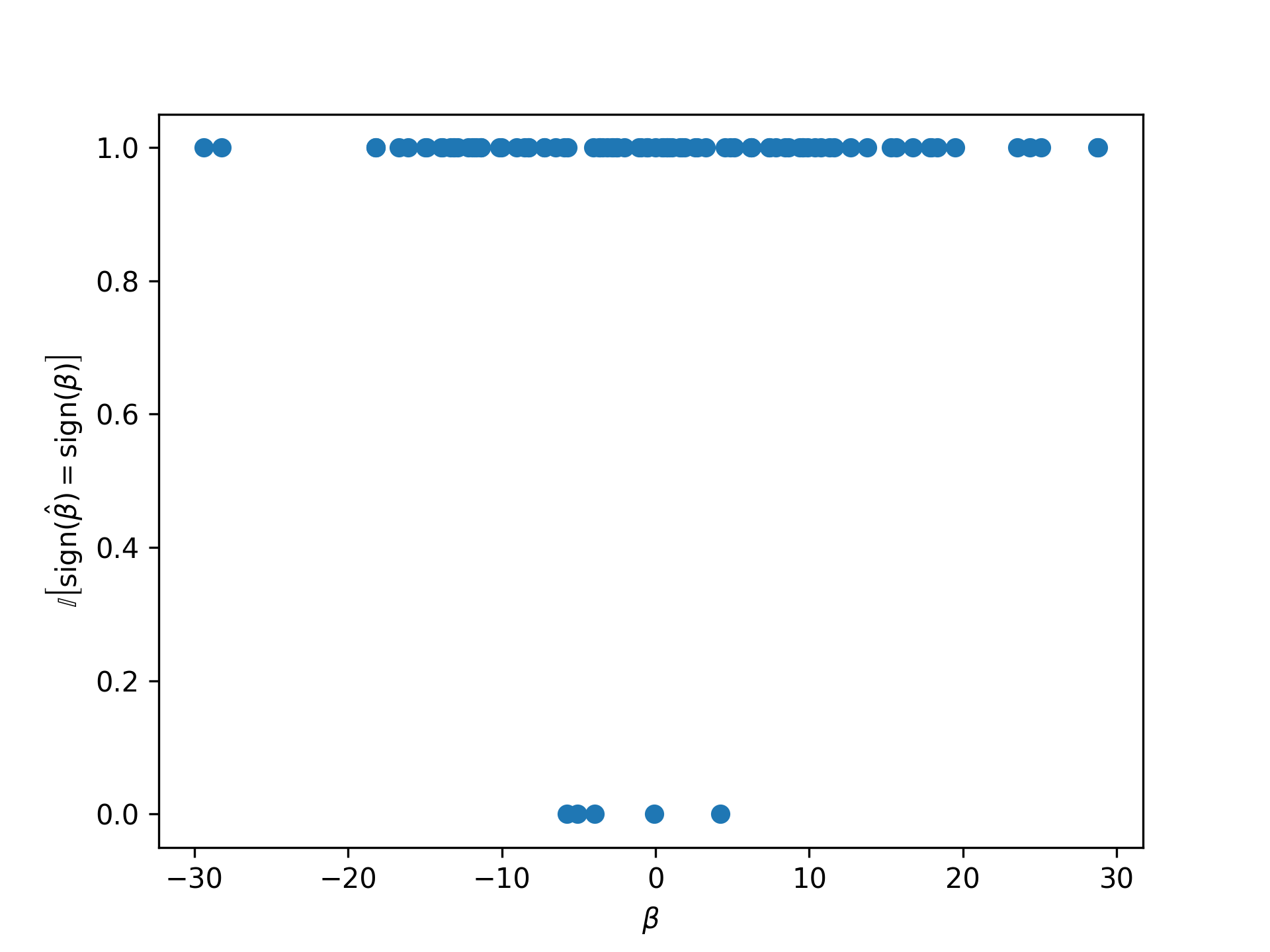
What is evident here is that when the rank-based SEM got the signum wrong it also tended to be the case that the absolute value of the true parameter was small. This isn’t particularly surprising, but also note that the misclassification only occurred a small number of times among the many parameters of the model.
I also noted that there is a substantial amount of correlation between the accuracy of the signum in the rank-based vs linear SEM, and that generally both approaches did a pretty good (albeit imperfect) job of recovering the signum. Below is a plot of these accuracies paired by the true data generating process that was used.
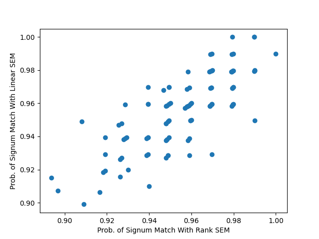
In this particular computational experiment I found that
\[\hat P \left[ \hat P \left[ \mathbb{I} \left[ \operatorname{sign} \left( \hat \beta_{\text{rank}} \right) = \operatorname{sign} \left( \beta \right) \right] \right] > \hat P \left[ \mathbb{I} \left[ \operatorname{sign} \left( \hat \beta_{\text{linear}} \right) = \operatorname{sign} \left( \beta \right) \right] \right] \right] = \frac{39}{100}\]
and
\[\hat P \left[ \hat P \left[ \mathbb{I} \left[ \operatorname{sign} \left( \hat \beta_{\text{linear}} \right) = \operatorname{sign} \left( \beta \right) \right] \right] > \hat P \left[ \mathbb{I} \left[ \operatorname{sign} \left( \hat \beta_{\text{rank}} \right) = \operatorname{sign} \left( \beta \right) \right] \right] \right] = \frac{35}{100}\]
which are close enough that 100 replicates could still easily be due to sampling variation. This is not strong evidence of stochastic dominance. Notably the rank-based SEM was not obviously dominated by the linear SEM in this experiment sampling from conditional normal variables.
As I discussed in Spearman Correlation Quantifies Comonotonicity, the notion of quantifying which variables go up-and-down together (or reverse) is valuable to scientists and other practitioners of statistics. With rank-based SEM we can hypothesize patterns of increasing/decreasing relationships among the variables according to a structural causal model.
Here is the code to replicate the experiment.
from itertools import product
import random
from time import ctime

import matplotlib.pyplot as plt
import networkx as nx
import numpy as np
import pandas as pd
from scipy.stats import rankdata
import semopy

# Utils


def decycle(d):
    """
    Pseudorandomly remove cycles from a directed graph.

    Changes the graph inplace.

    PARAMETERS
    ----------
    d : networkx.DiGraph
        Directed graph.

    RETURNS
    -------
    None
    """
    while True:
        if nx.is_directed_acyclic_graph(d):
            break
        first_cycle = nx.cycles.find_cycle(d)
        target_edge = random.sample(first_cycle, 1)[0]
        d.remove_edge(*target_edge)


rank = lambda x: rankdata(x, method="dense", axis=0)

# Config
k = 100
n = 100
m = 1000
possible_edges = list(product(range(n), repeat=2))
np.random.seed(2018)
linear_scores = []
rank_scores = []

for _ in range(k):
    # Generate a DAG
    d = nx.DiGraph()
    edges = random.sample(possible_edges, n)
    d.add_edges_from(edges)
    decycle(d)

    # Create Lavaan-style string following DAG
    model_str = ""
    for node in nx.topological_sort(d):
        node_str = f""
        for i, edge in enumerate(d.out_edges(node)):
            if i == 0:
                node_str += f"x{edge[1]}"
            else:
                node_str += f"+x{edge[1]}"
        if node_str:
            model_str += f"x{node} ~ {node_str}\n"

    ##    print(model_str)
    model = semopy.Model(model_str)

    # Generate data that follows DAG
    data = np.random.normal(size=m * n).reshape(m, n)
    betas = {edge: np.random.normal(scale=10) for edge in d.edges()}
    str_betas = {
        frozenset((f"x{k1}", f"x{k2}")): val for (k1, k2), val in betas.items()
    }
    for node in nx.topological_sort(d):
        for edge in d.out_edges(node):
            data[:, node] += betas[edge] * data[:, edge[1]]

    df = pd.DataFrame(data, columns=[f"x{i}" for i in range(n)])
    df_rank = pd.DataFrame(rank(data), columns=[f"x{i}" for i in range(n)])

    # Train model on data
    linear_results = model.fit(df)
    linear_inspection = model.inspect()

    linear_inspection = linear_inspection[linear_inspection["op"] == "~"]
    linear_inspection["true_beta"] = linear_inspection[
        linear_inspection["op"] == "~"
    ].apply(lambda row: str_betas[frozenset([row.rval, row.lval])], axis=1)
    linear_score = (
        linear_inspection["Estimate"].apply(np.sign)
        == linear_inspection["true_beta"].apply(np.sign)
    ).mean()
    linear_scores.append(linear_score)

    # Train model on ranks of data
    rank_results = model.fit(df_rank)
    rank_inspection = model.inspect()

    rank_inspection = rank_inspection[rank_inspection["op"] == "~"]
    rank_inspection["true_beta"] = rank_inspection[rank_inspection["op"] == "~"].apply(
        lambda row: str_betas[frozenset([row.rval, row.lval])], axis=1
    )
    rank_score = (
        rank_inspection["Estimate"].apply(np.sign)
        == rank_inspection["true_beta"].apply(np.sign)
    ).mean()
    rank_scores.append(rank_score)

    print(_, ctime(), linear_score, rank_score)

# Some plots
plt.scatter(
    rank_inspection["true_beta"],
    rank_inspection["Estimate"].apply(np.sign)
    == rank_inspection["true_beta"].apply(np.sign),
)
plt.xlabel(r"$\beta$")
plt.ylabel(
    r"$\mathbb{I} \left[ \operatorname{sign}(\hat \beta) = \operatorname{sign}(\beta) \right]$"
)
plt.savefig("rank_sem_equal_signum_vs_param.png", dpi=300, transparent=True)
plt.close()

plt.scatter(rank_scores, linear_scores)
plt.xlabel("Prob. of Signum Match With Rank SEM")
plt.ylabel("Prob. of Signum Match With Linear SEM")
plt.savefig("prob_signum_match_sem.png", transparent=True)
plt.close()
Discussion & Conclusions
I was able to show that rank-based SEM is pretty good at recovering the signum of the true parameters from a family of data generating processes. Because the underlying process had only conditionally linear parameters, the recovery of the signum of the parameters also meant that the rank-based SEM was telling us about monotonicity. However, the coefficients in the rank-based model would tell us about monotonicity in many cases anyway.
This is still quite a limited example because many data generating processes will not be conditionally Gaussian, but it is a good first approximation. Likewise the true data generating process that I used is linear in its path functions, but that is not necessary. A further example where the true path functions are non-linear in the parameters would make for a more interesting example. What I expect is that the rank-based SEM will tend to recover the conditionally-dependent monotonicity when it is strong in tendency, although not necessarily the signum of any parameters in the path functions as they may not so simply relate to the monotonicity relationship as was the case in linear SEM.