import numpy as np
from matplotlib import pyplot as plt
from typing import List

def simulate_ar(
    intercept: float,
    coefs: List[float],
    noise: float = 0.3,
    warmup: int = 10,
    steps: int = 200,
    rng=None
    ) -> np.ndarray:
    """Simulates an autoregressive (AR) time series.

    Args:
        intercept (float): The intercept term of the AR process.
        coefs (List[float]): List of coefficients for the lagged terms.
        noise (float, optional): The standard deviation of the Gaussian noise. Default is 0.3.
        warmup (int, optional): Number of initial steps to discard to allow the process to stabilize. Default is 10.
        steps (int, optional): Number of steps to simulate after the warmup period. Default is 200.

    Returns:
        np.ndarray: Simulated AR time series data of length `steps`.
    """
    rng = np.random.default_rng() if rng is None else rng
    max_lag = len(coefs)
    draws = np.zeros(warmup + steps)
    draws[:max_lag] = intercept
    for step in range(max_lag, warmup + steps):
        draws[step] = intercept + rng.normal(0, noise)
        for lag, coef in enumerate(coefs, start=1):
            draws[step] += coef * draws[step - lag]
return draws[warmup:]How to Naïvely Generate Autoregressive Time Series Data in Python
Python
Statistics
Stochastic Processes
Autoregressive
Time Series
Matplotlib
NumPy
In this post I will show you how to simulate an autoregressive (AR) process using Matplotlib and NumPy.
First, let’s define a function which pseudorandomly generates the data sequence. We’ll set an intercept parameter to set a consistent offset of the series from zero, and a sequence of autoregressive coefficients. The order of the coefficients entails the lag order that they are each applied to, so if you want to skip a lag order you can just set it to zero. Some AR series are noisier than others, and you can set that level of noise using the noise parameter. In this model we assume that the noise is a stationary normal distribution:
\[\epsilon_t \sim \mathcal{N}(0,\sigma)\]
for all \(t\).
The following implementation is a generalization of the implementation provided in Generate Fake Autoregressive Data in which I have allowed for any number of time lags. I have also allowed a user-provided random number generator to be passed.
Let us set a seed for reproducibility.
RANDOM_SEED = 2018
rng = np.random.default_rng(RANDOM_SEED)
Now let’s choose some parameters.
# True parameters of the AR process
intercept = 10
coefs = [-0.3, 0.1, -0.3]  # Example coefficients for AR process with 3 lags
Now let us simulate the AR process.
ar_data = simulate_ar(intercept, coefs, warmup=2018, steps=200, rng=rng)Finally, let us plot the simulated data using Matplotlib.
fig, ax = plt.subplots(figsize=(8, 3))
ax.set_title("Generated Autoregressive Timeseries", fontsize=15)
ax.plot(ar_data)
ax.set_xlabel('Time')
ax.set_ylabel('Signal')
plt.show()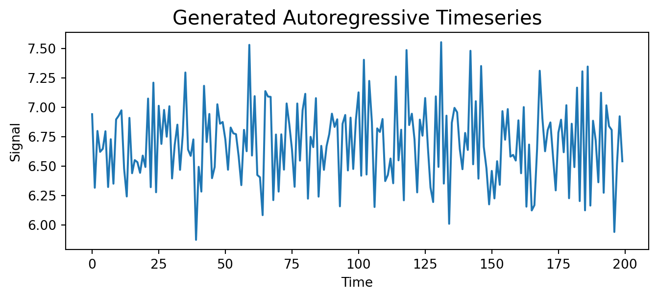
This implementation is not particularly efficient in terms of computing resources. Although performance is influenced by many things, a large factor is the presence of an ordinary for loop. Upon every iteration of the loop the Python interpreter will check that all types are still valid, which is a waste of computing resources when you can assume that they are. Perhaps I will write a more efficient function, but this example should be suitable for examples and tinkering for now.
Here is the output data for the example:
ar_dataarray([6.941708 , 6.3155875 , 6.79896769, 6.62115125, 6.64690478,
6.79654732, 6.32163015, 6.72852581, 6.35004628, 6.89721308,
6.92979629, 6.97466588, 6.47919687, 6.24134393, 6.91045418,
6.43927381, 6.55083547, 6.53331397, 6.44255904, 6.58915744,
6.4923775 , 7.07488836, 6.32039603, 7.21035304, 6.27709664,
7.0134047 , 6.68872494, 6.97816857, 6.75025929, 7.00950853,
6.39465926, 6.68118717, 6.85268958, 6.46779684, 6.76181945,
7.29674199, 6.64142503, 6.58699206, 6.72707155, 5.87192126,
6.49363922, 6.28287734, 7.18342675, 6.70507765, 6.94382677,
6.39717353, 6.49306093, 7.02621907, 6.8610425 , 6.87523356,
6.7267247 , 6.46888024, 6.8280871 , 6.7789368 , 6.77176061,
6.58257732, 6.33784174, 6.808397 , 6.62658717, 7.53212642,
6.59001865, 7.09541224, 6.4240351 , 6.40443905, 6.08217251,
7.13828813, 7.09221513, 7.08928927, 6.21026942, 6.76872715,
6.28272682, 6.77029136, 6.46984318, 7.0331383 , 6.85807573,
6.64286023, 6.3238929 , 7.03278515, 6.54674528, 6.97528036,
7.11517396, 6.22263056, 6.74882539, 6.66139963, 7.0783666 ,
6.23980551, 6.67212967, 6.46792713, 6.66990209, 6.77251836,
6.94614928, 6.83357381, 6.89816709, 6.15734245, 6.86025094,
6.93488203, 6.46304183, 6.91241082, 6.47560317, 6.89390062,
7.12772216, 6.41811335, 7.40498293, 6.42844055, 7.2251552 ,
6.87492573, 6.15158164, 6.82079686, 6.790811 , 6.90070107,
6.37238571, 6.42500936, 6.56438666, 6.35378324, 7.26239073,
6.54888149, 6.80957892, 6.20860224, 7.48779131, 6.84955546,
6.94570356, 6.72697226, 6.27613628, 6.89544594, 6.75888508,
7.07931692, 6.66666166, 6.3180758 , 6.19398727, 7.09355878,
6.49304741, 7.55478488, 6.35099042, 6.92931065, 6.00868397,
6.86902339, 6.99545602, 6.95783505, 6.64467603, 6.47337945,
6.78201172, 6.63753378, 7.48158873, 6.51522663, 7.05250727,
6.39296225, 7.3519113 , 6.66425586, 6.48041592, 6.17408598,
6.45883478, 6.22486773, 6.54137246, 6.34066406, 6.96759892,
6.72473722, 6.98529234, 6.58060658, 6.59542768, 6.54721287,
6.88949907, 6.43898143, 7.00231541, 6.1544984 , 6.68328599,
6.12233025, 6.16702292, 6.64338878, 7.31158216, 6.90580583,
6.62631565, 6.80756359, 6.87177271, 6.57651991, 6.29329644,
6.78533065, 6.8948178 , 6.61792592, 7.0182514 , 6.22628874,
6.86051622, 6.49121734, 7.16799008, 6.20211378, 7.30671013,
6.12323977, 7.34758837, 6.16358606, 6.88596075, 6.71944393,
6.36211338, 7.12466492, 6.27294854, 7.01723785, 6.84008439,
6.80771285, 5.93900768, 6.51765076, 6.92400731, 6.54072599])