Implementing a G/G/1 Queue in Ciw

Introduction

Ciw is a Python package for simulating queueing networks.

The two G’s in G/G/1 do not have to be the same distribution, and respectively can be any distribution with non-negative support.

We will use a Hyperexponential distribution for the arrival distribution. A hyperexponential distribution is exactly a mixture distribution of exponential distributions. This has an interpretation of there being an implicit set of arrival processes that each have their own distinct but independent exponential arrival times. In this case we will choose a mixture of four such arrival processes with distinct arrival rates:

\[\begin{align} U_1 \sim & \text{Exponential}\left( \frac{1}{9} \right) \\ U_2 \sim & \text{Exponential}\left( \frac{1}{5} \right) \\ U_3 \sim & \text{Exponential}\left( \frac{1}{6} \right) \\ U_4 \sim & \text{Exponential}\left( 1 \right) \end{align}\]

The following mixture distribution for the arrival times will be used:

\[T_{\text{arrivals}} \sim \frac{1}{5} f_{U_1} + \frac{1}{10} f_{U_2} + \frac{3}{5} f_{U_3} + \frac{1}{10} f_{U_4}\]

We will use a gamma distribution for the sake of example. A gamma distribution is the result of a sum of independent exponentially-distributed random variable, and thus for this example we have an interpretation that the servicing is implicitly a multi-step process where each step has an exponentially-distributed completion time.

Simulation

A G/G/1 queue as described can be implemented and simulated using Ciw in the following way.

import ciw

ciw.seed(2018)

arrival_dist = ciw.dists.HyperExponential(rates=[9, 5, 6, 1], probs=[0.2, 0.1, 0.6, 0.1])
service_dist = ciw.dists.Gamma(shape=0.6, scale=1.2)
HORIZON = 365

network = ciw.create_network(
    arrival_distributions = [arrival_dist],
    service_distributions = [service_dist],
    number_of_servers = [1]
    )
    
simulation = ciw.Simulation(network)
simulation.simulate_until_max_time(HORIZON)
records = simulation.get_all_records()

Results

We can tabulate the results.

from IPython.display import Markdown, display
import pandas as pd
records = pd.DataFrame(records)
display(
    Markdown(
        records
        [['waiting_time', 'service_time', 'queue_size_at_arrival', 'queue_size_at_departure']]
        .describe()
        .to_markdown()
        )
    )

	waiting_time	service_time	queue_size_at_arrival	queue_size_at_departure
count	546	546	546	546
mean	118.578	0.668262	176.855	510.295
std	64.0327	0.813994	103.554	289.318
min	0	9.40731e-07	0	7
25%	66.9117	0.0991315	87	258
50%	119.865	0.348732	177.5	527.5
75%	175.243	0.901602	270.75	763.5
max	224.18	4.88812	352	1015

We can plot the arrival times against the waiting times.

records.plot(x='arrival_date', y='waiting_time')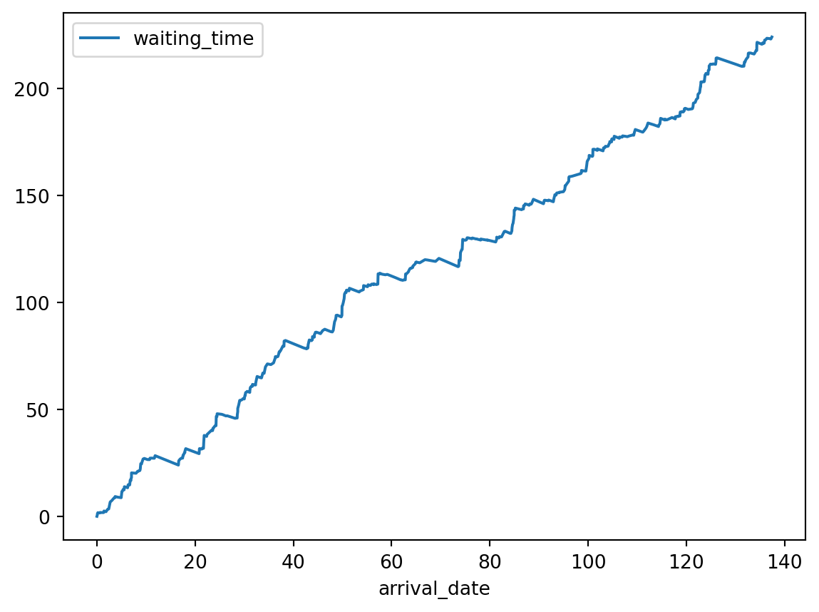

We can plot the service start times against the service times.

records.plot(x='service_start_date', y='service_time')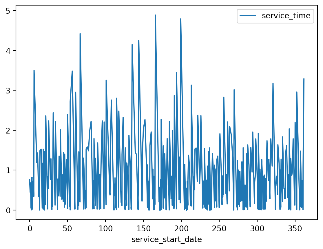

We can plot the arrival dates against the length of the queue when the customer arrived.

records.plot(x='arrival_date', y='queue_size_at_arrival')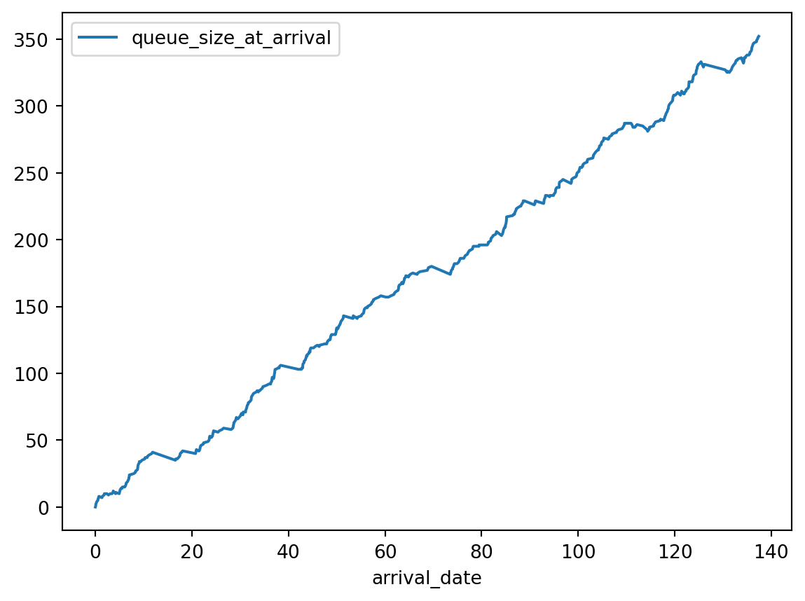

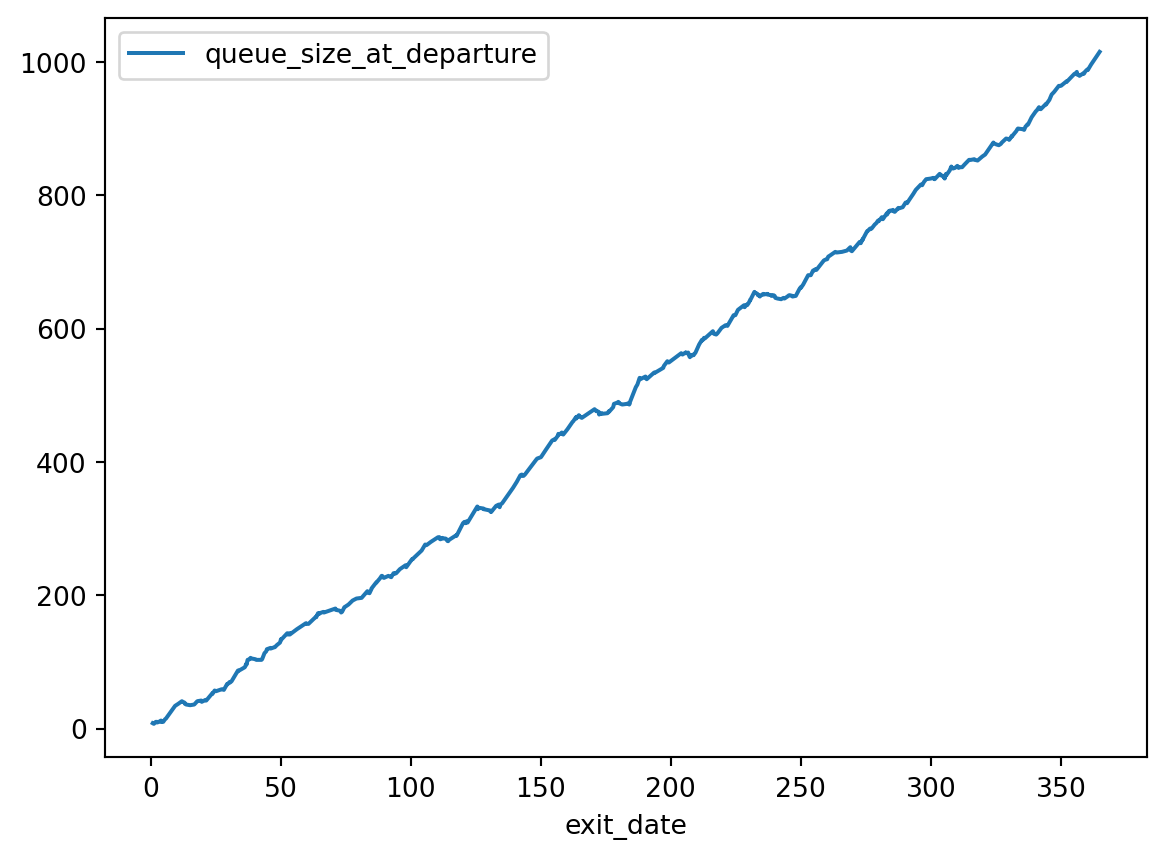
We can plot the departure dates against the length of the queue when the customer departed.

records.plot(x='exit_date', y='queue_size_at_departure')