Notes on Differential Forms

Mathematics
Differential Forms
Author

Galen Seilis

Published

February 25, 2023

Modified

August 10, 2024

Tangent Space

Definition

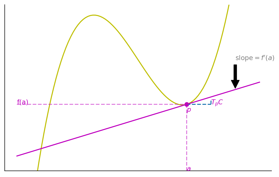
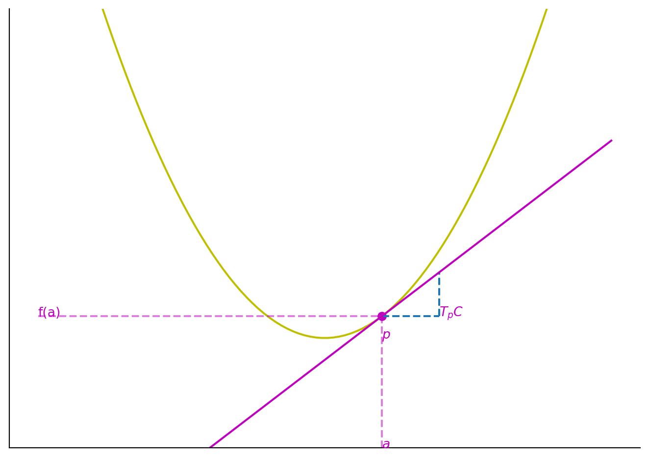
Suppose \(C \subseteq \mathbb{R}^2\) is a curve and \(p \in C\). The tangent space to \(C\) at \(p\), \(T_pC\) is the set of all vectors tangent to \(C\) at \(p\).

Example

Let us say we have a curve \[y = f(x)\], with a point \[p = (a, f(a))\]. A tangent vector at that point can be given by \[\vec v = \langle 1, f^{\prime}(a) \rangle\] where \[\langle \cdot, \cdot \rangle\] is an inner product. Then we can formulate the tangent space

\[T_pC = \text{span} \{ \langle 1, f^{\prime} \rangle \} = \{ \langle c, c f^{\prime}(a) | c \in \mathbb{R} \}.\]

import matplotlib.pyplot as plt
import numpy as np
fig = plt.figure()
ax = fig.add_axes((0.1, 0.2, 0.8, 0.7))
ax.spines[['top', 'right']].set_visible(False)
ax.set_xticks([])
ax.set_yticks([])
ax.set_ylim([-30, 15])
# Plot of function
x = np.linspace(-5, 5, num=100)
y = x ** 3 - 10 * x
ax.plot(x, y, color='y')
# Unit tangent vector
ax.plot([2,3], [-12]*2, '--', color='tab:blue')
ax.plot([3,3], [-11, -12], '--', color='tab:blue')
# Tangent space
ax.plot(x, 2 * x - 16, color='m')
ax.text(3, -12, r'$T_pC$', color='m')
ax.scatter(2, -12, color='m')
ax.text(2, -14, r'$p$', color='m')
ax.annotate(r'slope$=f^{\prime}(a)$', xy=(4, -8), xytext=(4, 0),
             arrowprops=dict(facecolor='black', shrink=0.05), color='grey')
# Pullbacks
ax.plot([2]*2, [-30,-12], '--', color='m', alpha=0.5)
ax.text(2, -30, r'$a$', color='m')
ax.plot([x.min(), 2], [-12]*2, '--', color='m', alpha=0.5)
ax.text(x.min(), -12, 'f(a)', color='m');

How do we differentiate between points on \(C \subseteq \mathbb{R}^2\) and vectors in \(T_p C \subseteq \mathbb{R}^2\)?

We can create a coordinate system on \(C\)

\[(x,y): C \mapsto \mathbb{R}^2\]

\[(x,y)(p) = (x(p), y(p))\]

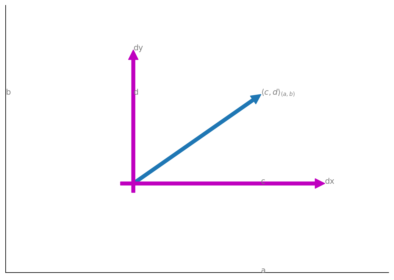
and a coordinate system on \(T_p C\):

\[\langle dx, dy \rangle : T_p C \mapsto \mathbb{R}^r\]

\[\langle dx, dy \rangle = \langle dx(v), dy(v) \rangle\]

Thus \(x: C \mapsto \mathbb{R}\) and \(y: C \mapsto \mathbb{R}\) are combined to get a coordinate vector in the ambient space.

Similarly, \(dx: T_pC \mapsto \mathbb{R}\) and \(dy: T_pC \mapsto \mathbb{R}\) are combined to get a coordinate vector in the tangent space.

Example

Let \(y = x^2\), then the coordinate vector is \((x,y)(p) = (a, a^2) \in C\). Similarly \(\langle dx, dy \rangle (v) = \langle 1, 2a \rangle \in T_pC\) where \(v\) is a tangent vector to the function.

import matplotlib.pyplot as plt
import numpy as np
fig, ax = plt.subplots()
ax.spines[['top', 'right']].set_visible(False)
ax.set_xticks([])
ax.set_yticks([])
ax.set_ylim([-5, 15])
# Plot of function
x = np.linspace(-5, 5, num=100)
y = x**2
ax.plot(x, y, color='y')
# Unit tangent vector
ax.plot([2,2], [1,3], '--', color='tab:blue')
ax.plot([1,2], [1, 1], '--', color='tab:blue')
# Tangent space
ax.plot(x, 2 * x - 1 , color='m')
ax.text(2, 1, r'$T_pC$', color='m')
ax.scatter(1, 1, color='m')
ax.text(1, 0, r'$p$', color='m')
# Pullbacks
ax.plot([1]*2, [-5,1], '--', color='m', alpha=0.5)
ax.text(1, -5, r'$a$', color='m')
ax.plot([-5, 1], [1]*2, '--', color='m', alpha=0.5)
ax.text(-5, 1, 'f(a)', color='m')
plt.tight_layout()

The equation \(\langle dx, dy \rangle (v) = \langle 1, 2a \rangle\) implies familiar result that \(dy = 2a \cdot 1 = 2 a dx \implies \frac{dy}{dx} = 2a = f^{\prime}(a).\)

Example

Note that \[\mathbb{R}^2 = \text{span} \{ (1,0), (0,1) \} = \{ (x,y) | x,y \in \mathbb{R} \}.\]

That means that

\[T_p \mathbb{R}^2 = \text{span} \{ \langle 1, 0 \rangle, \langle 0, 1 \rangle \} = \{ \langle dx, dy \rangle | dx, dy \in \mathbb{R} \}.\]

Tip

If you want to keep track of the tangent space at different points, you can denote \(\langle dx, dy \rangle_p\) for the tangent space at point \(p\).

Example

Suppose we have \(\langle 1, 2 \rangle_{(1,1)}\), we can think of the differentials as another set of axes as visualized below.

import matplotlib.pyplot as plt
import numpy as np
fig, ax = plt.subplots()
ax.spines[['top', 'right']].set_visible(False)
ax.set_xticks([])
ax.set_yticks([])
ax.set_xlim([0,3])
ax.set_ylim([0,3])
ax.annotate("", xy=(2,2), xytext=(1, 1),
            arrowprops=dict(color='tab:blue'))
plt.text(2, 2, r'$\langle c,d \rangle_{(a,b)}$', color='gray')
ax.annotate("", xy=(1,2.5), xytext=(1, 0.9),
            arrowprops=dict(color='m'))
ax.annotate("", xy=(2.5,1), xytext=(0.9, 1),
            arrowprops=dict(color='m'))
ax.text(2.5, 1, 'dx', color='grey')
ax.text(1, 2.5, 'dy', color='grey')
ax.text(2, 1, 'c', color='grey')
ax.text(1, 2, 'd', color='grey')
ax.text(2, 0, 'a', color='grey')
ax.text(0, 2, 'b', color='grey')
plt.tight_layout()

1-Forms

Definition

A 1-form is a linear function \(\omega : T_p \mathbb{R}^n \mapsto \mathbb{R}\).

Proposition

For a 1-form \(\omega : T_p \mathbb{R}^n \mapsto \mathbb{R}\) it holds that \(\omega \in (T_p \mathbb{R})^{*}\) where \((T_p \mathbb{R})^{*}\) is the dual space of the tangent space \(T_p \mathbb{R}\).

Example

Given \(\mathbb{R}^2\) and \(T_p \mathbb{R}^2\) and \(\omega : T_p \mathbb{R}^2 \mapsto \mathbb{R}\) be linear:

\[\implies \omega (\langle dx, dy \rangle) = adx + bdx = \langle a, b \rangle \cdot \langle dx, dy \rangle\]

which also equals

\[\vert| \langle a, b \rangle \vert| \operatorname{scalar\_projection}_{\langle a,b \rangle} \langle dx, dy \rangle .\]

This leads to an intuition that a 1-form is a multiple of the scalar projection on to the same line.

Example

Let \(\omega : T_p \mathbb{R}^n \mapsto \mathbb{R}\) then

\[\omega ( \langle dx_1, \ldots, dx_n \rangle ) = \sum_{i=1}^n a_i dx_i\]

Example

Define \(\omega (\langle dx, dy \rangle) = 3dx + 2dy.\) What line does \(\omega\) project vectors onto?

  • The line is in the direction \(\langle 3, 2 \rangle\) b/c \(\omega ( \langle dx, dy \rangle ) = \langle 3,2 \rangle \cdot \langle dx, dy \rangle\)

Notice that \(\langle 3,2 \rangle\) is parallel to \(\langle 1, \frac{2}{3} \rangle\) which entails that \(dy = \frac{2}{3} x.\)

Example

Suppose \(\omega\) scalar projects onto the line \(dy = 2dx\) with length of 3. Find \(\omega .\)

We know that \(\omega (\langle dx, dy \rangle) = \langle a,b \rangle \cdot \langle dx, dy \rangle .\) We need \(\langle a, b \rangle\) to be parallel to \(\langle 1, 2 \rangle\) because \(\langle 1, 2 \rangle\) is the vector in the direction of the line \(dy = 2dx\).

So \(\langle a, b \rangle = \langle a, 2a \rangle\) which needs that have \[\vert| \langle a, 2a \rangle \vert| = 3 \] .

So \[\vert| \langle a, 2a \rangle \vert| = \sqrt{a^2 + 4 a^2} = 3 \implies a \sqrt{5} = 3 \implies a = \frac{3}{\sqrt{5}}\] . So \(b=\frac{6}{\sqrt{5}}\)

\[\implies \omega (\langle dx, dy \rangle) = \frac{3}{\sqrt{5}} dx + \frac{6}{\sqrt{5}} dy\]

Example

Supposing \(n=2\) and \(\omega_1 \wedge \omega_2 : T_p \mathbb{R}^2 \times T_p \mathbb{R}^2 \mapsto \mathbb{R}\) then what is \(\omega_1 \wedge \omega_2 (v_1, v_2)\) where \(v_1, v_2 \in \mathbb{R}^2\) ?

References