How Expressive Are Simple Neural Networks?

It is well-known that neural networks are universal function approximators under mild assumptions. Such theorems proving arbitrary bounds on the empirical risk and similar results tell us that a good approximation exists. They do not tell us how readily neural networks will approximate other functions in practice. The last few decades have shown that neural networks can be hugely successful on complicated domains such as images, audio and text.

But still I do not have refined intuitions for just how good/bad neural networks are when they are simple. The common approach of building neural networks that are more complicated than needed but are then regularized to prevent overfitting is obviously useful, but it has done little to understand the boundary where they break down. That is, except for a few classic examples such as learn the XOR function with a single hidden layer in a multi-layer perceptron.

In keeping with that theme of tinkering with simple scenarios to gain intuitions about the fundamentals, I decided to train some multilayer perceptrons are some elementary functions.

The following script generated noiseless data sets representing systematic samplings of functions such as \(\sin\), \(\cos\), \(\tan\), \(e^t\), \(2t+3\), and a few polynomials. The data was normalized in the domain (within the model) and image (outside of the model) of the estimand functions to reduce the effects of differing location and scale. That is to say, I was more interested in the learnability of “shape” up-to-but-not-including location and scale. For each data set a sequence of multilayer perceptrons were trained on it with increasing width in the hidden layer. Finally, plots were generated to understand the training behaviour and the visual goodness of fit. For these examples I am only interested in the models’ ability to fit a given pattern, but not whether it generalizes well.

import matplotlib.pyplot as plt
import tensorflow as tf

# Utility

def tfnormalize(x):
    return (x - tf.reduce_mean(x)) /\
           tf.math.reduce_variance(x)

# MLP factory
def genmlp(width):
    '''
    width: width of internal layer.
    '''
    model = tf.keras.models.Sequential()
    model.add(tf.keras.Input(shape=(1,)))
    model.add(tf.keras.layers.Normalization())
    model.add(tf.keras.layers.Dense(width, activation='sigmoid'))
    model.add(tf.keras.layers.Dense(1))
    return model
    

# Prepare data
t = tf.linspace(-10, 10, num=10**4)
t = tf.reshape(t, shape=(-1,1))
functions = {
    'sine':tf.sin,
    'cosine':tf.cos,
    'tan':tf.tan,
    'exponential':tf.exp,
    'linear':lambda x: 2*x+3,
    'quadratic':lambda x: tf.pow(x,2),
    'cubic':lambda x: tf.pow(x,3),
    'quartic':lambda x: tf.pow(x,4),
    'abs':tf.abs
    }
images = {key:f(t) for key,f in functions.items()}
images = {key:tfnormalize(ft) for key,ft in images.items()}

# Train models
results = {}
models = {}
widths = list(range(1,11))
for func in functions:
    results[func] = {}
    models[func] = {}
    y = images[func]
    for w in widths:
        print(func, w)
        models[func][w] = genmlp(w)
        models[func][w].compile(optimizer='adam',loss='mse')
        history = models[func][w].fit(x=t, y=y, epochs=100)
        results[func][w] = history.history['loss']


# Plot results
for func in results:
    fig, axis = plt.subplots()
    axis.set_title(func)
    for w in results[func]:
        plt.plot(results[func][w], label=str(w))
    axis.set_yscale('log')
    fig.legend()
    plt.savefig(f'{func}_training_history.png', dpi=300, transparent=True)
    plt.close()

# Plot model predictions
for func in models:
    fig, axis = plt.subplots()
    axis.set_title(func)
    axis.plot(t, images[func], label='True', color='k')
    for w in models[func]:
        axis.plot(t, models[func][w].predict(t), label=str(w))
    fig.legend()
    plt.savefig(f'{func}_visual_fit.png', dpi=300, transparent=True)
    plt.close()

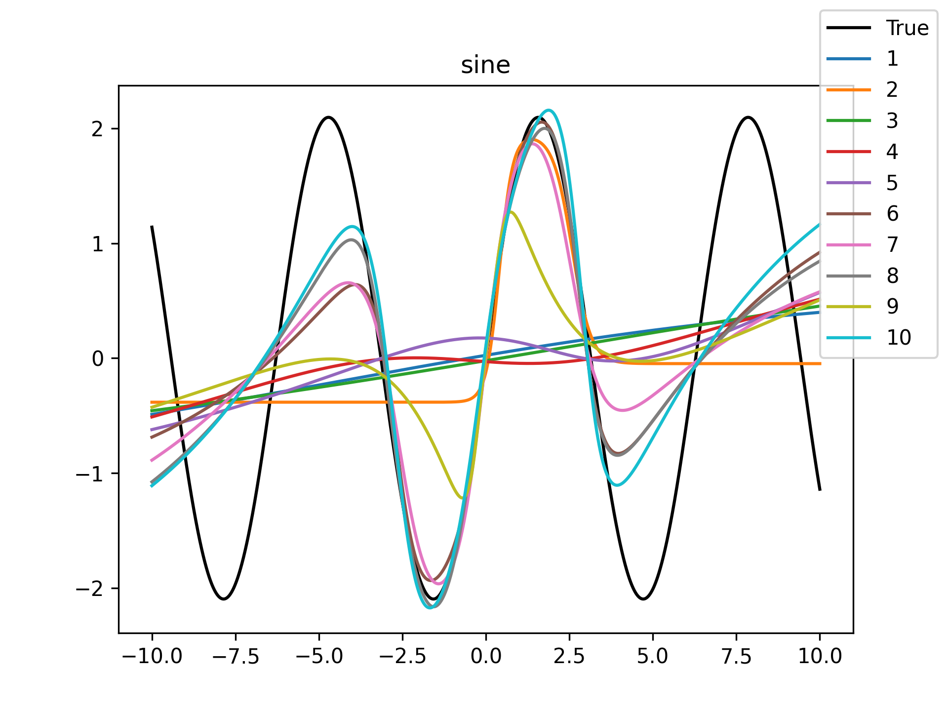
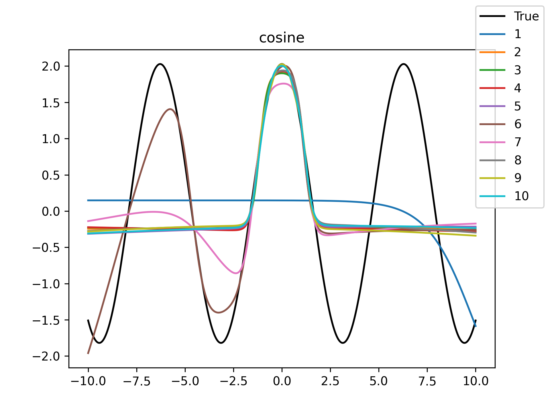
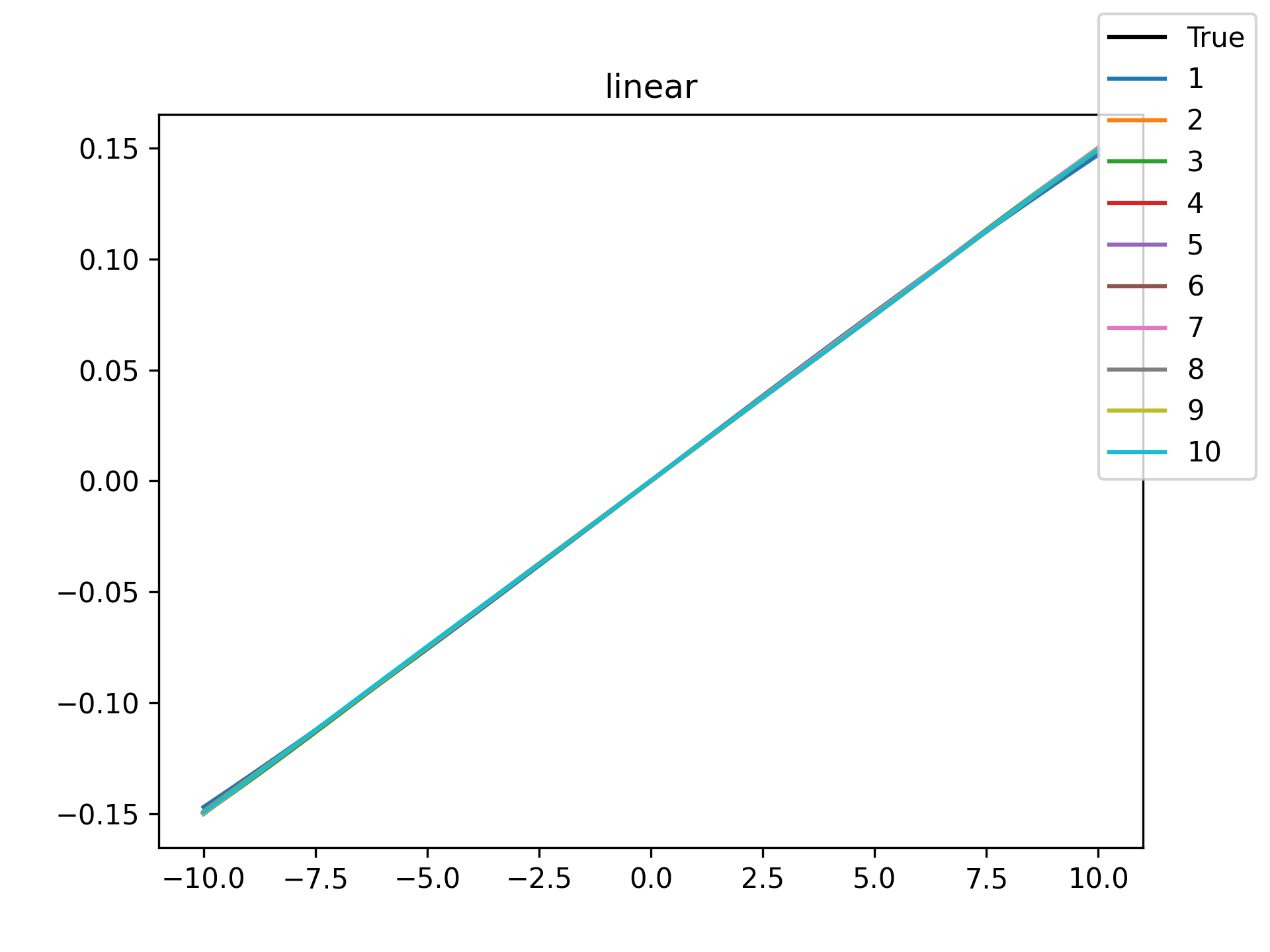
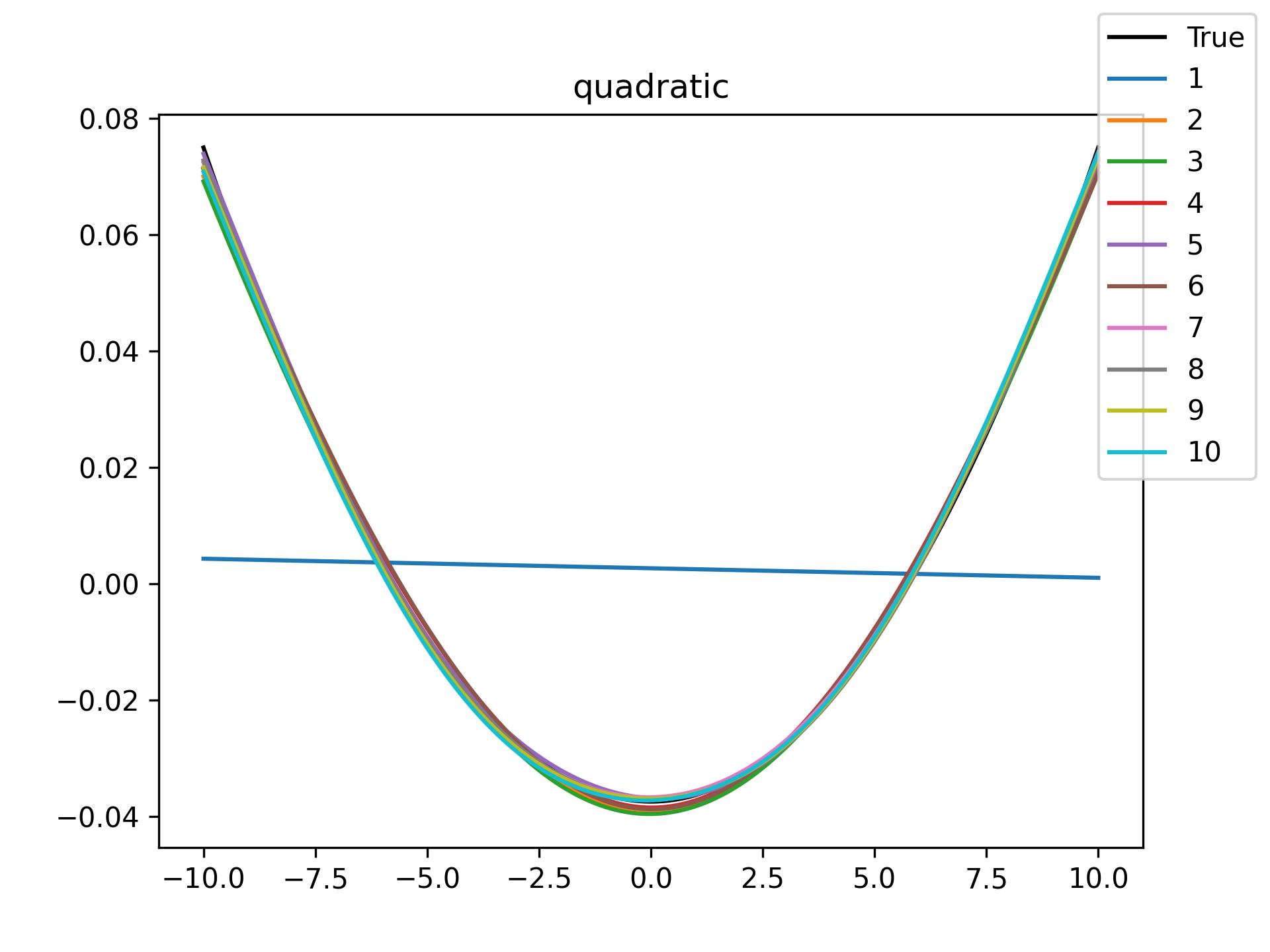
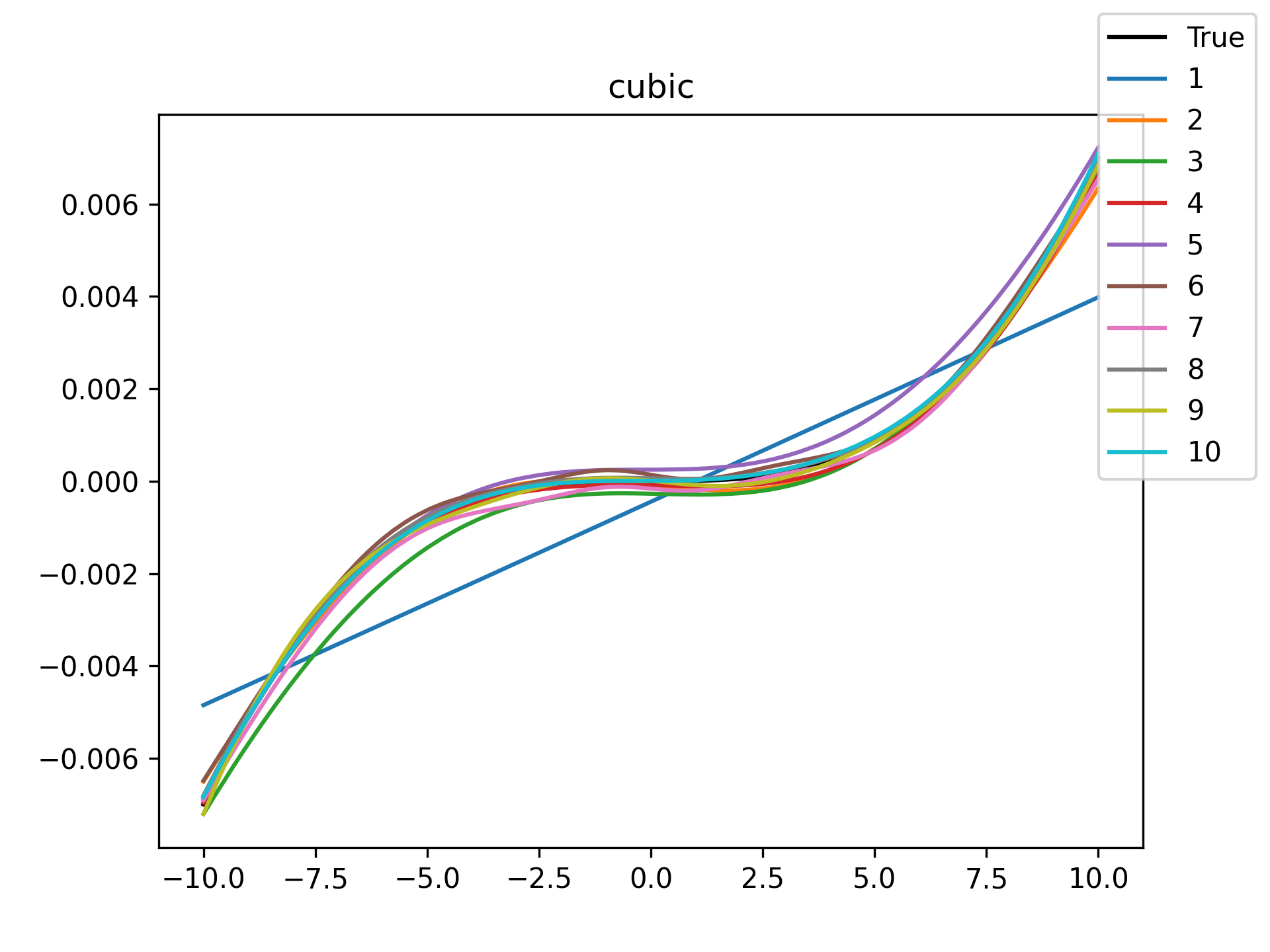
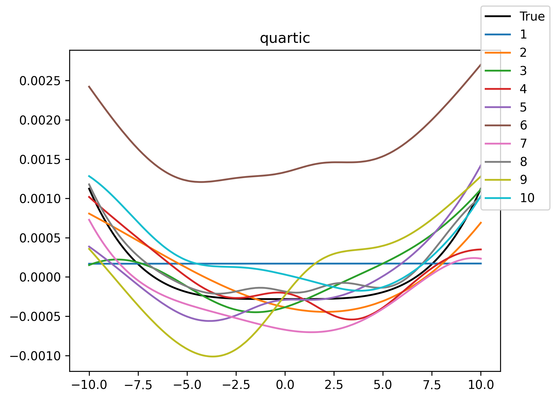
The following table of figures summarizes the results.

Function	Training History	Visual Fit
sin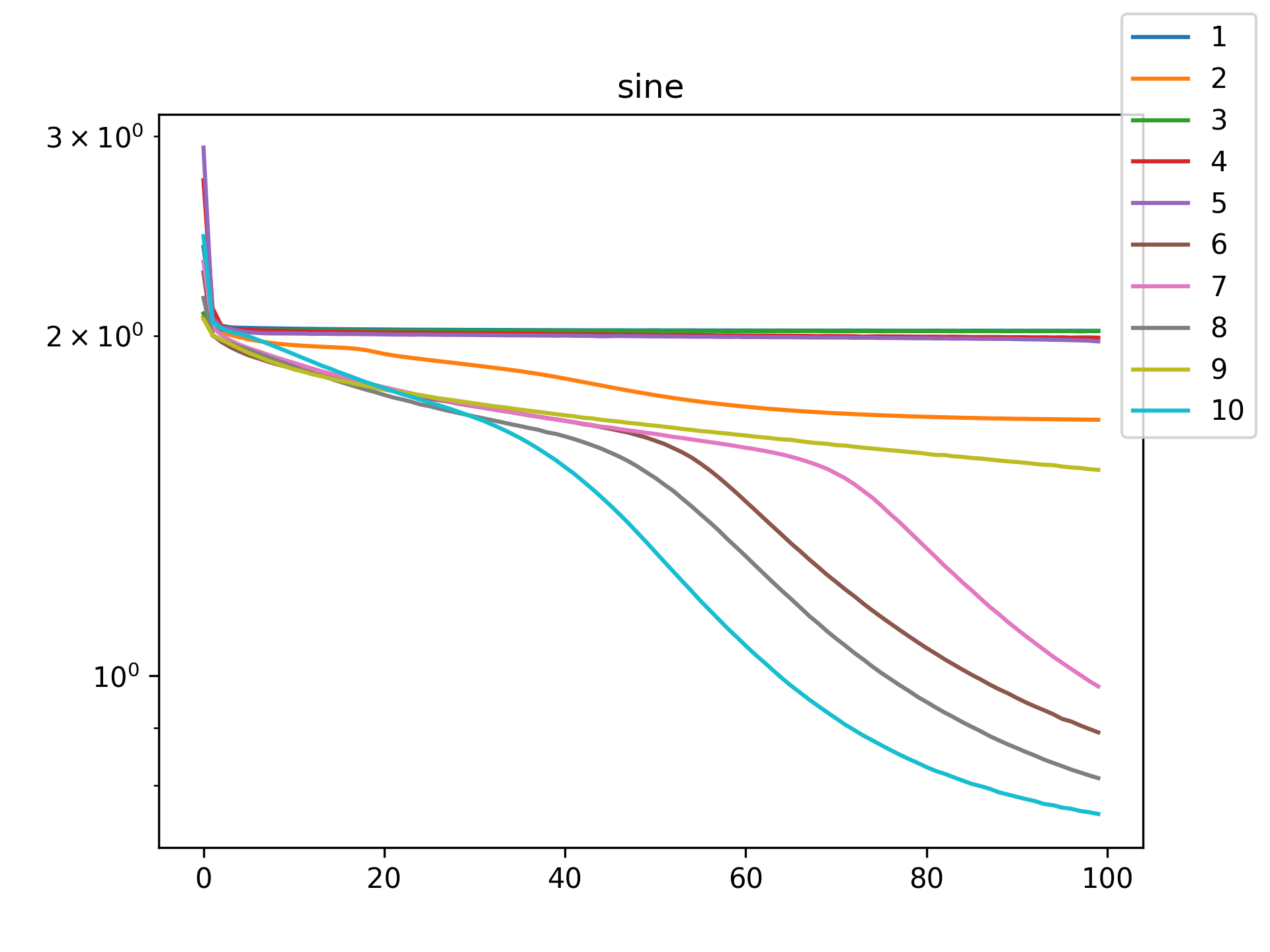
cos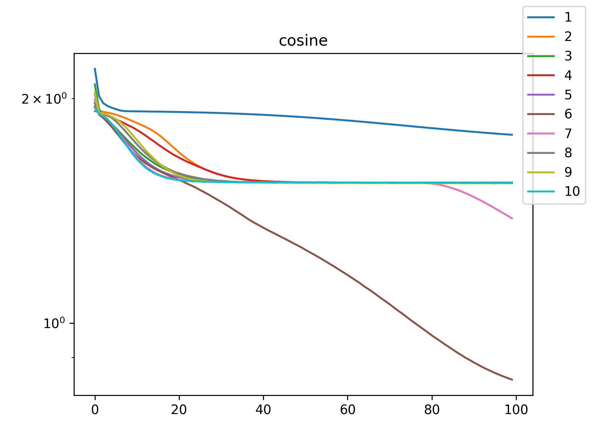
tan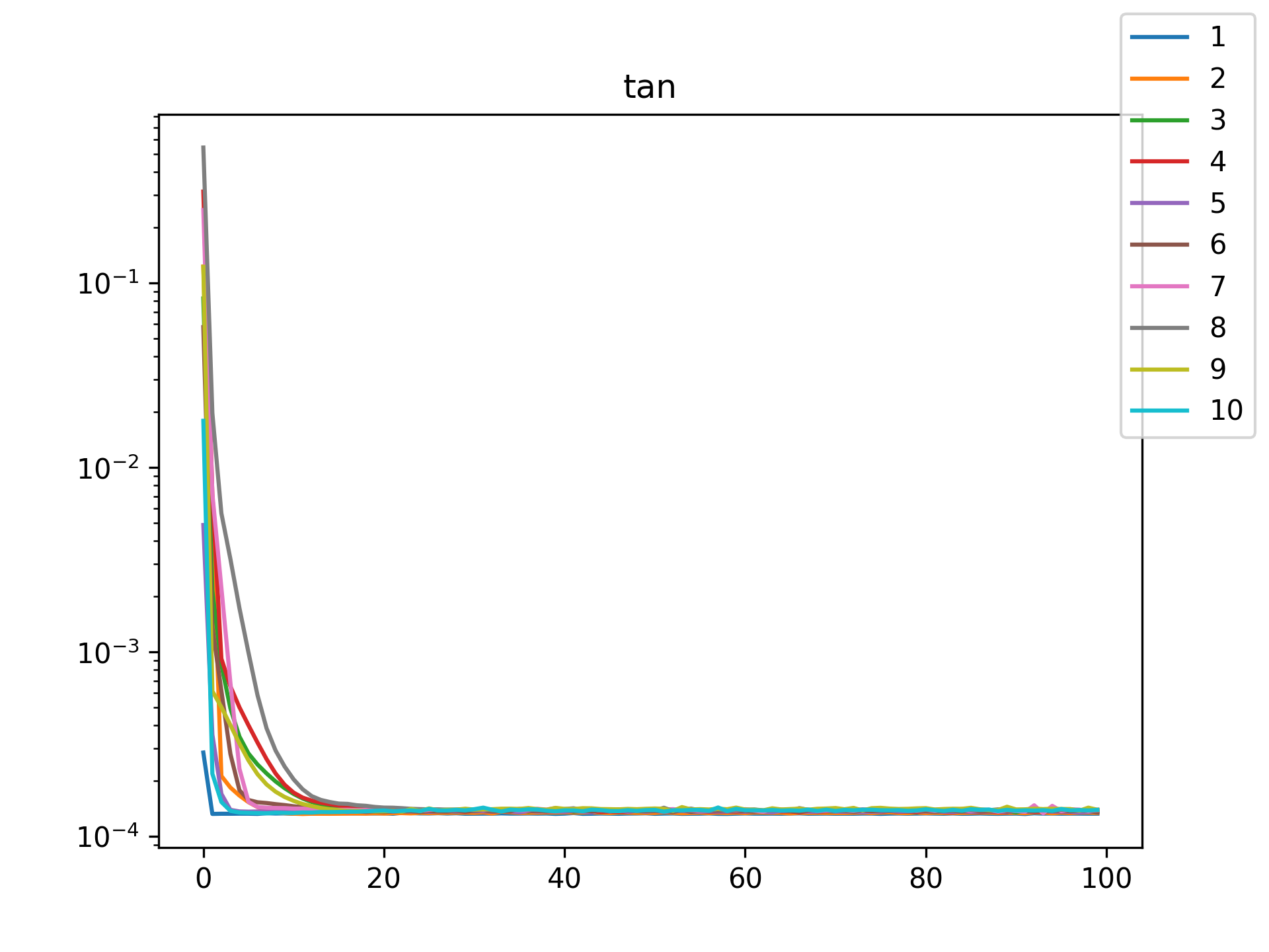
exponential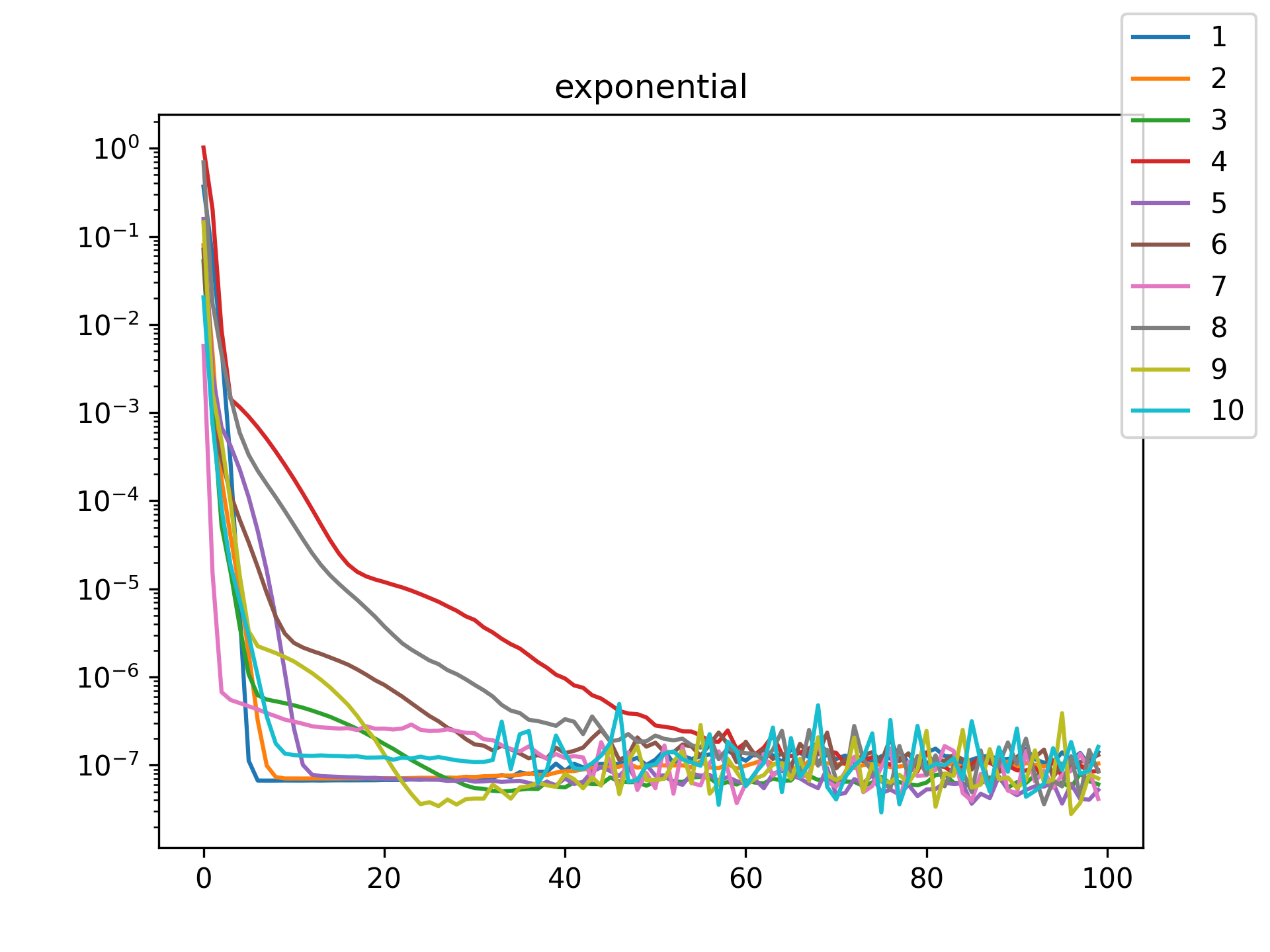
linear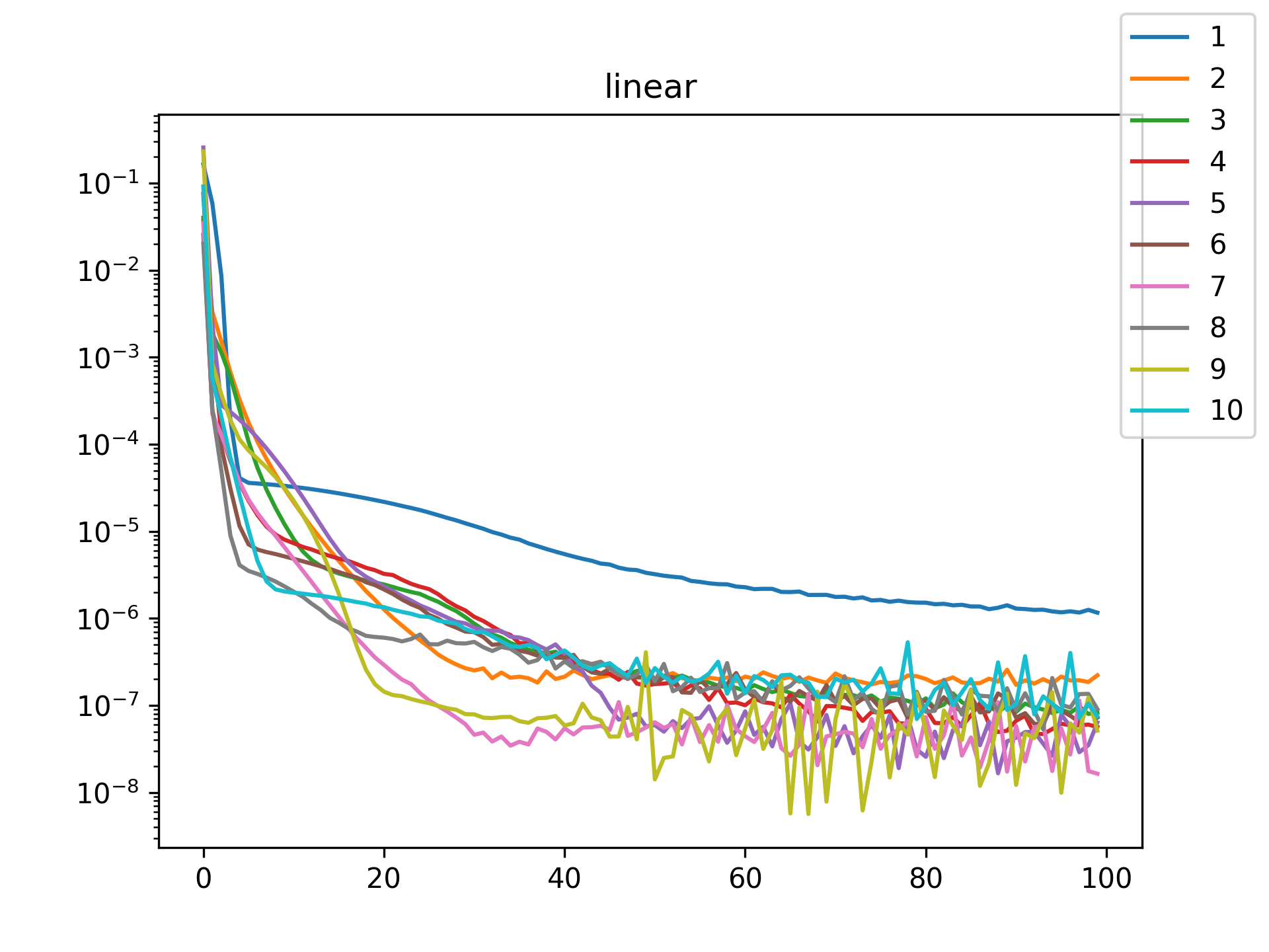
quadratic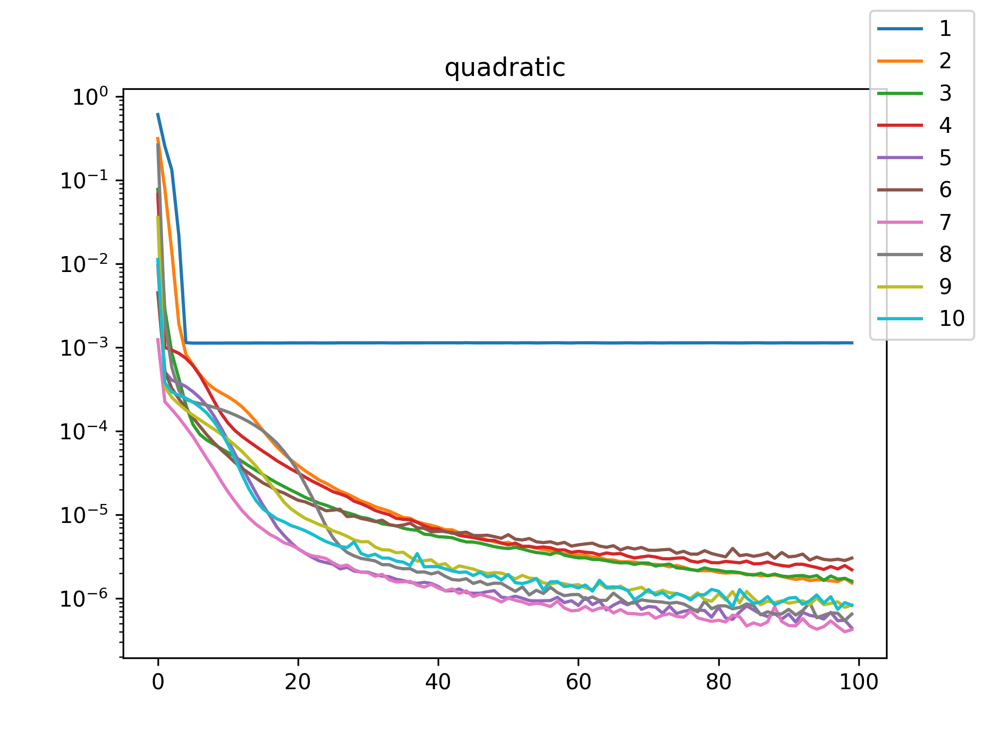
cubic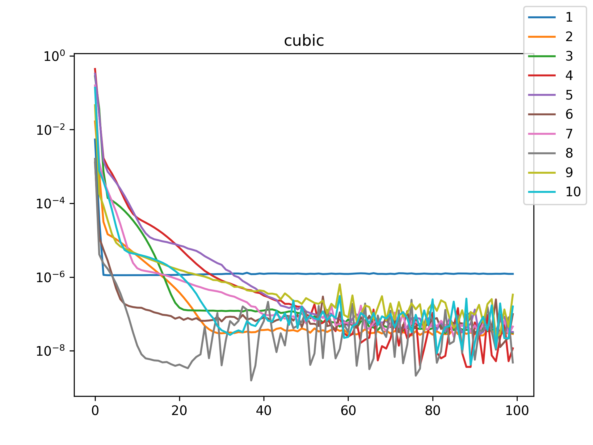
quartic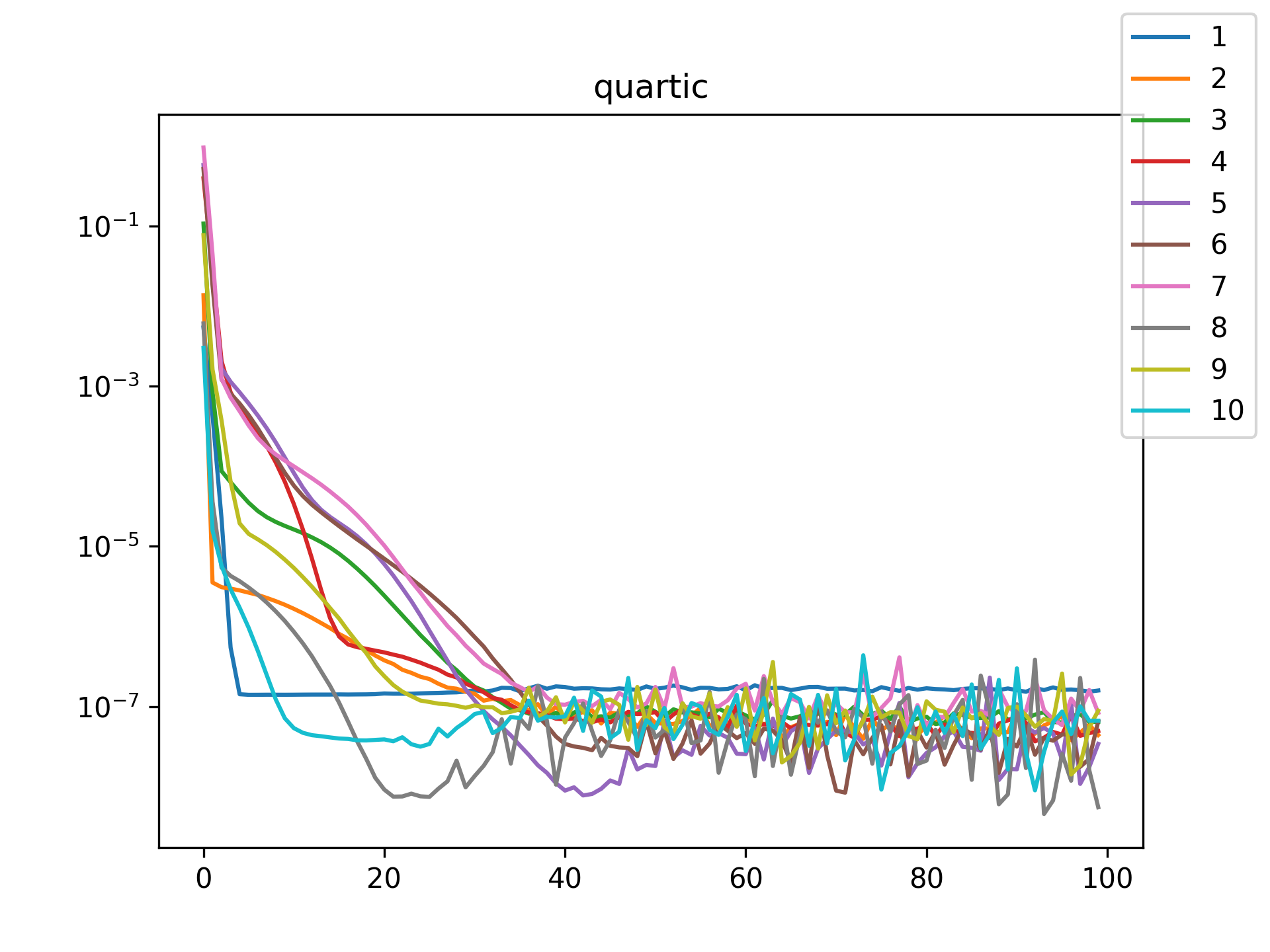
abs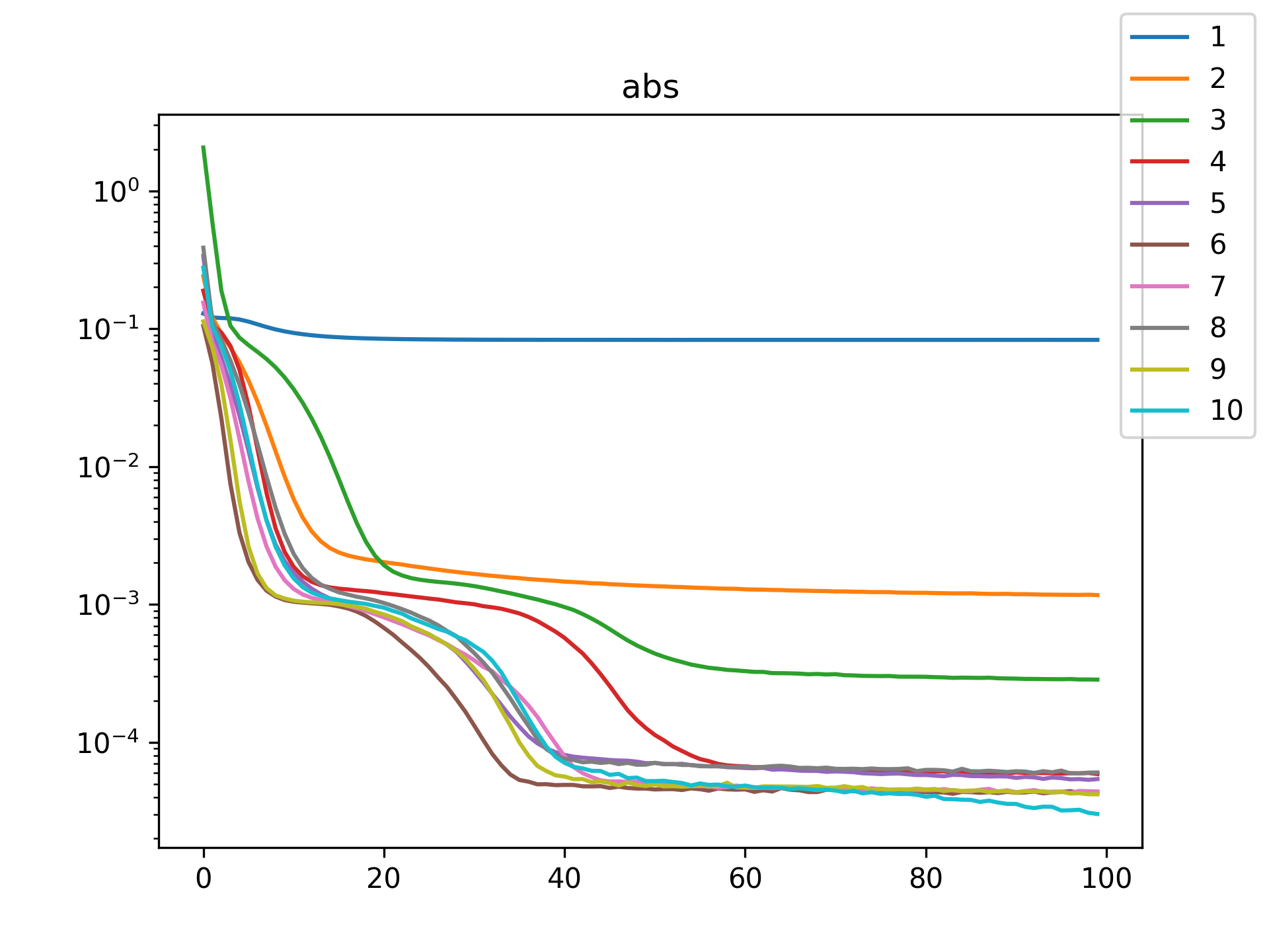

I see in the training histories that there is noisiness in some of the loss updates, suggesting that some combination of step size or numerical precision could be at play. Probably the former I suspect since the error is not especially close to the machine epsilon around \(10^{-16}\). In some cases such as the linear function it may just be that the gradient is more-or-less flat since the visual goodness of fit is excellent even for a single neuron.

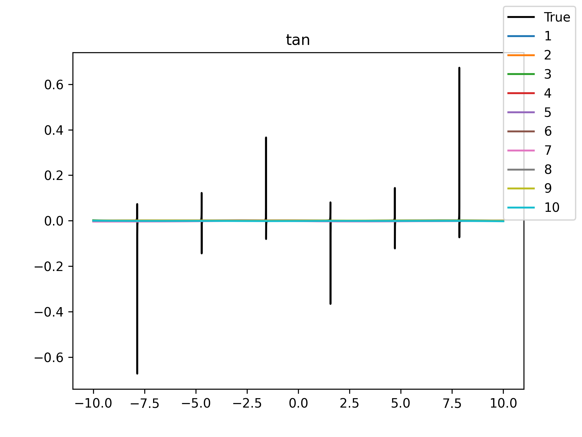
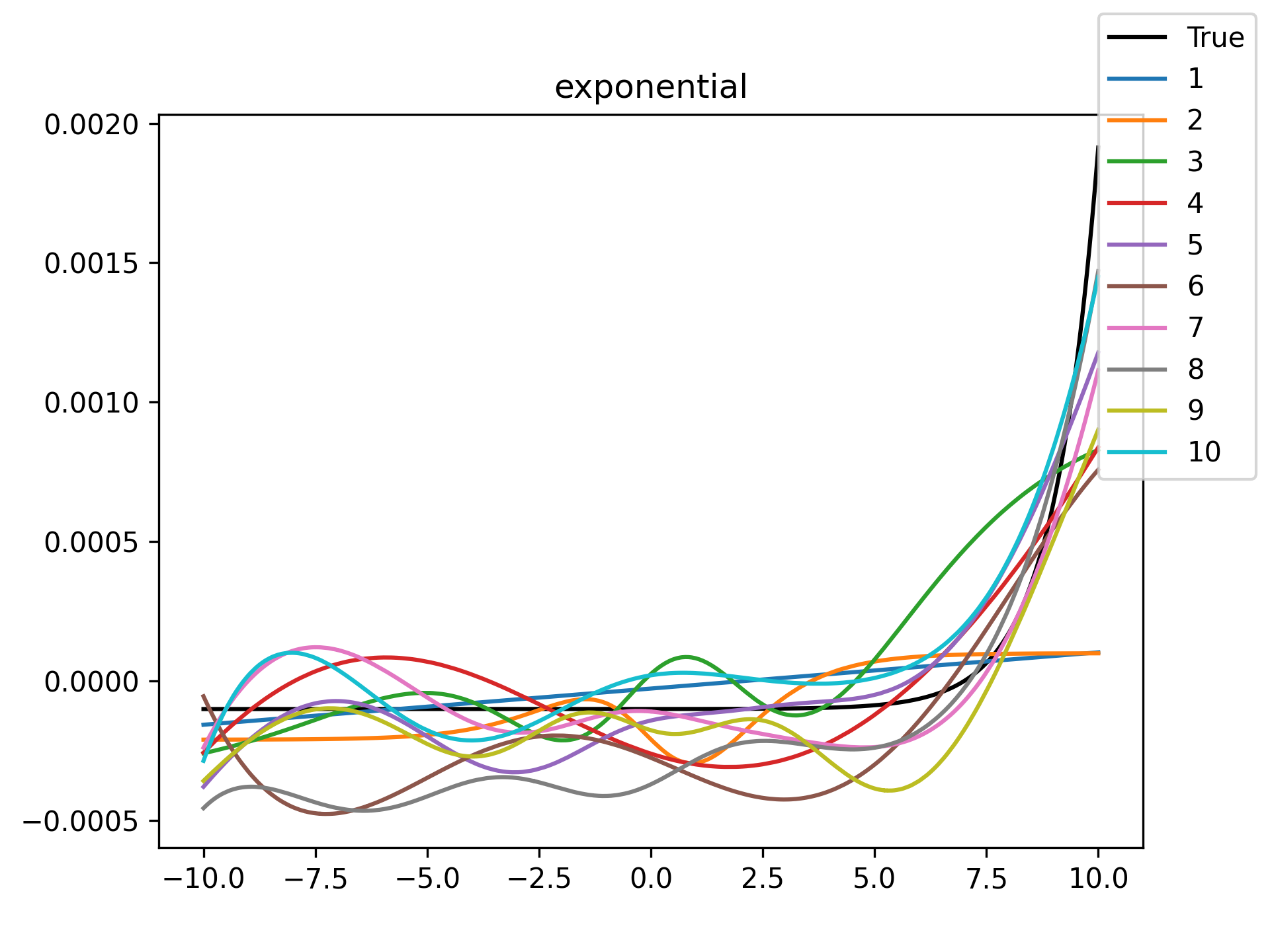
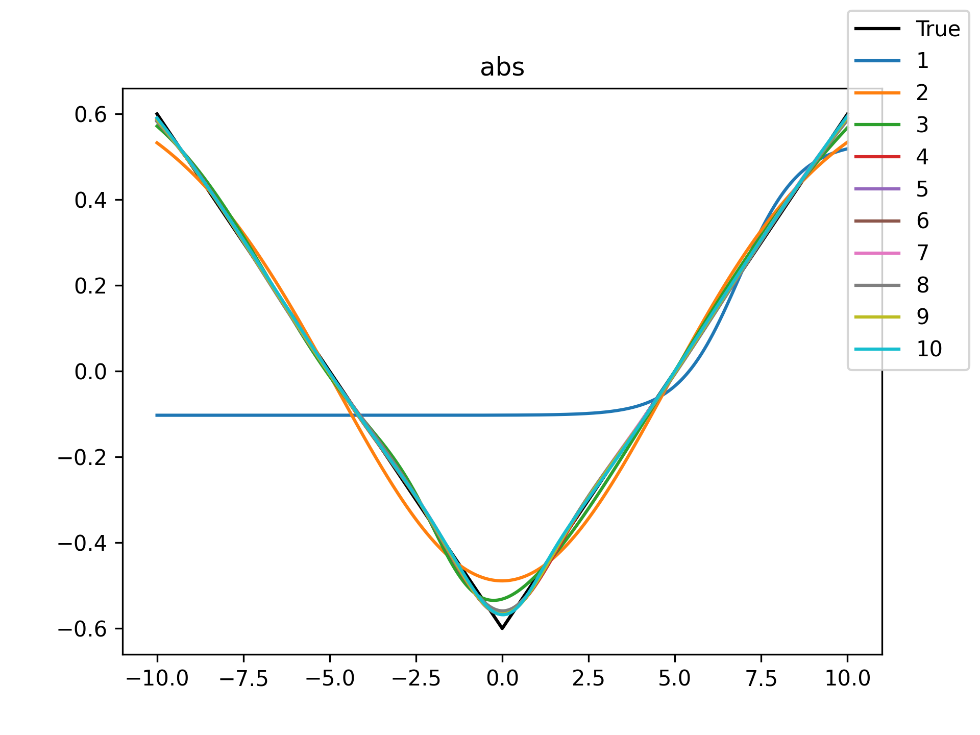
Unsurprisingly the models with only a single hidden neuron did poorly whenever there was a substantial bend in the data, but in many cases they substantially improved with only a handful more neurons. The only function where the networks made little improvement on approximating was the tangent function, which even after normalization still gives really sharp turns in the data that are not easily learned by these simple neural networks. The next-worst were the other sinusoids sine and cosine. While sine and cosine don’t have discontinuities, they do pose a challenge because their curvature periodically changes sign. Sigmoid functions a monotonic, so just to acheive a single pattern of down-up or up-down requires at least two neurons. With periodic functions over the real number line there is a need for an infinite number of such turns… But taking the modulus \(2 \pi\) in some cases could vastly simplify what the model has to learn. Then again, if you know that all you have a superposition of waves on a fixed interval then you might as well use Fourier series. But then again, ‘again’, you could say that for any of these functions. Neural networks will always perform no-better than the ground truth, and that their main selling point is approximating a function when you do not know it.

Now, it is worth noting that this demonstration doesn’t provide much in the way of highly general inferences. There are many choices to how I setup this experiment that could be tweaked in ways that improve or worsen the fit of the neural networks. But still, I find seeing examples adds an extra level of (hopefully not misleading) intution about what things can look like.

On the whole of it, I’m impressed at what even a small number of hidden neurons can accomplish. We often don’t get to see these examples because when the estimand functions are so simple we don’t usually both with neural networks. It was interesting for me to just take a peak this idealized case for intuition.