Minimal Bayesian Von Mises Model Example

Found this code in my miscellaneous bin folder. Instead of deleting it I thought I would share it here. It is a minimal working example of using the PyMC package to model a Von Mises distribution with priors put on its parameters. It is an extremely small model given by:

\[\kappa \sim \text{Exponential}(1)\]

\[\mu \sim \text{Uniform}\left( -\pi, \pi \right)\]

\[\theta \sim \text{VonMises}(\mu, \kappa)\]

And here is the aforementioned Python code:

"""CLI entry point."""

from __future__ import annotations

import sys

import arviz as az
import matplotlib.pyplot as plt
import numpy as np
import pymc as pm

from minimal_von_mise_example.model import build_model


def main() -> int:
    """Run sampling and plot trace."""
    observed = np.array([-2] * 10 + [2] * 10)
    model = build_model(observed=observed)

    with model:
        data = pm.sample(chains=2, tune=10, draws=10, progressbar=False)
        az.plot_trace(data)
        plt.tight_layout()
        plt.show()
    return 0


if __name__ == "__main__":
    sys.exit(main())

I can see from observed=[-2]*10 + [2]*10 that I was tinkering with having data at exactly two angles. Maybe I was stress-testing the sampler for how it handles bimodality.

Here is an example output. Because I didn’t set a seed number you may find your plot differs from mine somewhat.

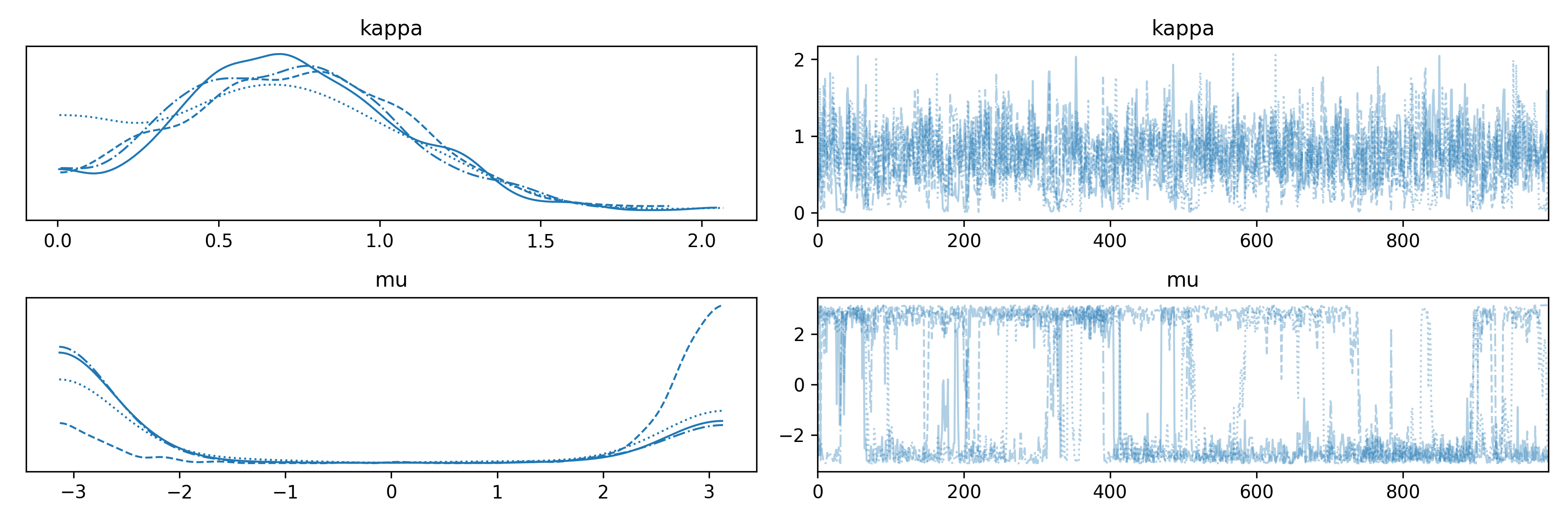
Adding az.summary(data, round_to=2).to_markdown('von_mise_bimdal_test.md') to the code above we can also see a summary of the model parameters. It is not a great effective sample size (ESS) and R-hat (\(\hat r\)), especially for \(\mu\). Actually, \(\kappa\) doesn’t look horrible despite the low ESS. The plot above also suggests that there are a couple of states that the chain switches between, which are likely the two modes.

	mean	sd	hdi_3%	hdi_97%	mcse_mean	mcse_sd	ess_bulk	ess_tail	r_hat
kappa	0.73	0.35	0.02	1.31	0.01	0.01	707.46	587.96	1
mu	0.79	2.65	-3.05	3.14	0.38	0.27	76.52	678.25	1.04

If I were to continue developing this model I would look at having a mixture distribution for \(\mu\). It would also be nice to get rid of that uniform prior on \(\mu\) by replacing it with something a little more informative.